OPEN ACCESS
In this paper the geometrical, optical and thermal study and simulation of a concentrator Linear Fresnel Reflector is carried out. Plant performances are analyzed through a mathematical calculation model that allows energy simulations to be made to estimate the productive effectiveness of the plant and to detect the temperature profiles of the various components subjected to concentrated solar radiation.
The absorption system was modeled using a finite difference discretization method. The implementation and resolution of the system of equations obtained, allows the causes of thermal and optical losses to be evaluated and the different types of orientation (North-South or East-West) to be compared by quantifying the energy productivity in the various cases on different days of the year.
The results derived from simulations show how the efficiency of the plant is influenced by some parameters that have been made to vary. In particular, the plant performance is strongly influenced by the index of emissivity of the selective coating that covers the absorber tube.
Concentrating solar power, Linear Fresnel, Finite-difference method.
A plant with linear Fresnel reflector is made up of a large number of mirrors that reflects and concentrates solar rays on a system of absorption, placed parallel to the rows of flat mirrors, a few meters from the ground [1]. The absorber is made up of a tube receiver and a secondary reflector which refocuses the beams towards the pipe. Inside the tube flows a heat transfer fluid which absorbs the energy and transports it to a heat exchanger for the production of steam, which subsequently expands in a steam turbine for the generation of electrical energy. Often, it also has a storage tank, which is necessary when moments of little or no solar radiation occur, as in the evening. The fluid used is composed of a mixture of molten salts that can be brought up to an operating temperature of 550 °C [2].
The requirement of only plane mirrors reduces costs with respect to the production and use of more complex geometries. For this reason this type of plant is named linear.
The primary reflectors are provided with one degree of freedom: the rotation around the axis parallel to the tube receiver. In the present work the analysis of the energy absorbing system modeling using finite difference discretization method, is carried out. With reference to a system installed at 40° N latitude, in addition to determining which orientation is more convenient, the aim is to identify which parameters have the greatest effect on yield.
Each row of mirrors must be inclined relative to the ground in such a way as the reflected beam is always incident on the receiver tube. Inclinations that assume the mirrors to concentrate the rays on the absorber tube are determined by the position of the sun is in the sky.
Figure 1. Schematization of the reflection on a panel
Figure 1 shows the three directions of the reflection represented by three unit vectors, respectively:
The laws of reflection provide two links between the unit vectors: they belong to the same plane and the angle between $\hat{n}$ and $\hat{n}_{t}$ and the one formed between $\hat{n}$ and $\hat{n}_{s}$ are congruent.
Through spherical trigonometry formulas it is possible to derive the relationship between the inclination of a generic reflector and solar coordinates [4]. Indicating with h the height at which the pipe absorber is installed relative to the axis of rotation of the mirror, the generic reflector is positioned at a distance D to the projection of the tube on plane x-y (Figure 2). The angle β which forms the normal to the horizontal direction East (Figure 2) is given by the following relationship:
$\beta=90^{\circ}-\arctan \frac{\sqrt{1-\cos ^{2} \phi \cos ^{2} a}-\sin \phi}{\cos \phi \sin a}+\frac{1}{2} \arctan \left(\frac{D}{h}\right)$(1)
Figure 2. Generic reflector
The term k, visible in Figure 1, is notably important. It is representative of the point where the reflected beam hits the absorption system. In fact, the point of arrival on the tube is not located at the same cross-section of the point at which the reflection occurs. With reference to the final part of the plant, it is often the case that the reflected rays, owing to this phase shift, do not affect the receiver. The length k, therefore, represents the plant portion in which the reflective surfaces do not provide useful effects. Its value can be obtained again using spherical trigonometry [4]:
$k=\frac{\cos \phi \cos a}{\sqrt{1-\cos ^{2} \phi \cos ^{2} a}} \cdot \sqrt{D^{2}+h^{2}}$(2)
The study is done using a calculation model that adequately describes the causes that affect the optical and thermal efficiency of these systems. The thermodynamic modeling has been developed for a concentrator with linear Fresnel mirrors, equipped with a tubular receiver and a secondary reflector.
3.1 Modeling of the absorption system
The absorber was discretized into n elements of constant length equal to Δx (Figure 3) [5].
Figure 3. Discretization along the longitudinal axis of the absorption system
The model was created to identify the thermal exchanges between the components of the absorber. Ignoring the radial conduction in metal and glass due to their small thickness, in each section four nodes are fixed to detect the temperatures of:
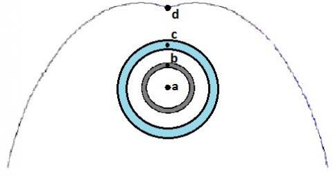
Figure 4 shows the discretization taken along the cross section of the absorption system.
Figure 4. Discretization along the cross section
With this discretization 4 x n nodes have been identified. The simplifying assumptions are:
For each node the energy balance equation has been written taking into account conductive, convective and radiative thermal exchanges between adjacent nodes at different temperatures.
$\left\{ \begin{align} & \dot{m}\ {{c}_{p}}\left( T_{a}^{i+1}-T_{a}^{i} \right)=\frac{T_{b}^{i}-T_{a}^{i}}{{{R}_{ab}}} \\ & \frac{T_{b}^{i}-T_{a}^{i}}{{{R}_{ab}}}+\frac{T_{b}^{i}-T_{c}^{i}}{{{R}_{irr,bc}}}+\frac{T_{b}^{i}-T_{b}^{i-1}}{{{R}_{cond,b}}}+\frac{T_{b}^{i}-T_{b}^{i+1}}{{{R}_{cond,b}}}={{{\dot{q}}}_{s,b}} \\ & \frac{T_{_{c}}^{i}-T_{b}^{i}}{{{R}_{irr,bc}}}+\frac{T_{c}^{i}-T_{d}^{i}}{{{R}_{irr,cd}}}+\frac{T_{c}^{i}-T_{c}^{i-1}}{{{R}_{cond,c}}}+\frac{T_{c}^{i}-T_{c}^{i+1}}{{{R}_{cond,c}}}+\frac{T_{_{c}}^{i}-{{T}_{ae}}}{{{R}_{e,c}}}={{{\dot{q}}}_{s,c}} \\ & \frac{T_{_{d}}^{i}-T_{c}^{i}}{{{R}_{irr,cd}}}+\frac{T_{d}^{i}-T_{d}^{i-1}}{{{R}_{cond,d}}}+\frac{T_{d}^{i}-T_{d}^{i+1}}{{{R}_{cond,d}}}+\frac{T_{_{d}}^{i}-{{T}_{ae}}}{{{R}_{e,d}}}={{{\dot{q}}}_{s,d}} \\ \end{align} \right.$ (3)
The meaning of the symbols used in the system of Eq. (3) is explained below.
Indicating the matrix of thermal conductances with ||G||, the vector of nodal temperatures with |T| and the vector of nodal flows with |F|, the system of equations is rewritten using in the following compact form:
$\left\| G \right\|\cdot \left| T \right|=\left| F \right|$ (4)
The vector of nodal temperatures is obtained by solving the system of equations by means of the inversion technique of the thermal conductance matrix.
3.2 Calculation of thermal resistance
3.2.1 Convective thermal resistance between the fluid and the inner tube Rab
$R_{a b}=\frac{1}{h_{i} \cdot \pi \cdot d_{b, \text { int }} \cdot \Delta x}$ (5)
in which the heat transfer coefficient between the fluid and the inner surface of the tube is indicated with hi; db,int is the internal diameter of the steel pipe, which is indicated by the subscript b. The estimation of the heat transfer coefficient is particularly complicated and affect much on the results of the simulation. To calculate this coefficient it is necessary to estimate the value of the Nusselt number in the case of forced convection for internal flow in ducts. The relationships used to estimate it [6] are a function of the Reynolds number and change according to the flow regime that is established inside the tube.
3.2.2 Axial conductive resistance of the steel pipe Rcond,b
${{R}_{cond,b}}=\frac{\Delta x}{{{\lambda }_{b}}\cdot \pi \cdot {{d}_{b,ave}}\cdot {{s}_{b}}}$ (6)
In the equation λb indicates the thermal conductivity of steel, db,ave and sb respectively indicate the average diameter and the thickness of the tube.
3.2.3 Axial conductive resistance of the outer glass Rcond,c
${{R}_{cond,c}}=\frac{\Delta x}{{{\lambda }_{c}}\cdot \pi \cdot {{d}_{c,ave}}\cdot {{s}_{c}}}$ (7)
In the equation λc indicates the thermal conductivity of glass, dc,ave and sc respectively indicate the average diameter and the thickness of the glass.
3.2.4 Radiative resistance between the two tubes Rirr,bc
The two tubes are coaxial and can be taken of infinite length; in the case of gray surfaces, the radiative thermal resistance is expressed as follows:
${{R}_{irr,bc}}=\frac{\frac{1}{{{\varepsilon }_{b}}}+\frac{1-{{\varepsilon }_{c}}}{{{\varepsilon }_{c}}}\frac{{{d}_{b,est}}}{{{d}_{c,\operatorname{int}}}}}{{{d}_{b,est}}\cdot \pi \cdot \Delta x\cdot \sigma \cdot \left( T_{b}^{2}+T_{c}^{2} \right)\cdot \left( {{T}_{b}}+{{T}_{c}} \right)}$ (8)
where εb and εc are the emissivity of the two cylinders; σ the constant of Stephan-Boltzmann and Tb and Tc the nodal temperatures.
3.2.5 Axial conductive resistance of secondary reflector Rcond,d
${{R}_{cond,d}}=\frac{\Delta x}{{{\lambda }_{d}}\cdot {{l}_{d}}\cdot {{s}_{d}}}$ (9)
In the equation λd indicates the thermal conductivity of the reflective material, ld and sd respectively indicate the curvilinear length and the thickness of the reflective surface.
3.2.6 Radiative resistance between the outer tube and the secondary reflector Rirr,cd
This resistance is a function of the view factor Fc-d between the outer surface of the absorber and the inner surface of the secondary reflector:
${{R}_{irr,cd}}=\frac{\frac{1-{{\varepsilon }_{c}}}{{{\varepsilon }_{c}}}+\frac{1}{{{F}_{c-d}}}+\frac{1-{{\varepsilon }_{d}}}{{{\varepsilon }_{d}}}\frac{{{A}_{c,est}}}{{{A}_{d}}}}{{{A}_{c,est}}\cdot \sigma \cdot \left( T_{c}^{2}+T_{d}^{2} \right)\cdot \left( {{T}_{c}}+{{T}_{d}} \right)}$ (10)
where Ac,estis the external area of an element of glass tube; εd and Ad = ld Δx are respectively the emissivity and the area of the element of the reflecting mirror.
3.2.7 External convective resistances Re,c and Re,d
The convective resistances between the glass and the air, and between the secondary reflector and the air, are respectively:
${{R}_{e,c}}=\frac{1}{{{h}_{e}}\cdot \pi \cdot {{d}_{c,est}}\cdot \Delta x}$ (11)
${{R}_{e,d}}=\frac{1}{{{h}_{e}}\cdot {{l}_{d}}\cdot \Delta x}$ (12)
where dc,est is the external diameter of the glass tube and he is the external heat transfer coefficient which depends on the type of convection that develops [6]. The he values are heavily determined by environmental conditions and, mainly, on the wind speed.
3.3 Calculation of solar powers
3.3.1 Solar Power absorbed by the secondary reflector \({{\dot{q}}_{s,d}}\)
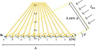
With the aid of the Figure 5 it is observed that the solar radiation directed towards the absorber system is equal to:
${{\dot{q}}_{r}}={{I}_{bn}}\cdot A\cdot \sin \phi \cdot {{\rho }_{RP}}$ (13)
where:
${{I}_{bn}}=A{{}_{1}}\cdot {{e}^{-\frac{{{A}_{2}}}{\sin \phi }}}$ (14)
where A1 and A2are respectively the apparent solar radiation outside the atmosphere and the atmospheric extinction coefficient;
$A=n{{}_{RP}}\cdot l\cdot \Delta x$ (15)
where nRP is the number of primary reflectors and l is their width;
Figure 5. Solar radiation reflected
The reflected radiation in part reaches the receiver tube directly and in part the secondary concentrator to then be reflected toward the tube. The ratio between the diameter of the receiver tube dc,est and the length of the aperture of the secondary reflector lap is called γ (Figure 6):
$\gamma=\frac{d_{c e s t}}{l_{a p}}$ (16)
Figure 6. Absorption system
The assumption made is that the concentrated radiation is distributed between the tube and the secondary reflector in a manner proportional to the diameter of the tube and the aperture of the reflector. The solar power absorbed by the node d is then:
${{\dot{q}}_{s,d}}={{\dot{q}}_{r}}\left( 1-\gamma \right){{\alpha }_{d}}={{I}_{bn}}{{n}_{RP}}\cdot l\cdot \Delta x\cdot \sin \phi \cdot {{\rho }_{RP}}\left( 1-\gamma \right)\cdot {{\alpha }_{d}}$ (17)
where αd is the absorptivity of the secondary reflector.
3.3.2 Solar power absorbed from the glass envelope \({{\dot{q}}_{s,c}}\)
The solar radiation absorbed by the glass tube comes in part directly from the primary reflectors and in part from the secondary reflector. It is therefore:
${{\dot{q}}_{s,c}}={{I}_{bn}}\cdot {{n}_{RP}}\cdot l\cdot \Delta x\cdot \sin \phi \cdot {{\rho }_{RP}}\cdot {{\alpha }_{c}}\left[ \gamma +\left( 1-\gamma \right){{\rho }_{d}} \right]$ (18)
where ρd is the reflectance of the secondary reflector and αc is the absorptivity of the glass tube.
3.3.3 Solar power absorbed by the steel tube \({{\dot{q}}_{s,b}}\)
The solar radiation that reaches the inner tube is given by two components: one coming from the mirrors and the other coming from the secondary concentrator:
${{\dot{q}}_{s,b}}={{I}_{bn}}\cdot {{n}_{RP}}\cdot l\cdot \Delta x\cdot \sin \phi \cdot {{\rho }_{RP}}\cdot {{\tau }_{c}}\cdot {{\alpha }_{b}}\left[ \gamma +\left( 1-\gamma \right){{\rho }_{d}} \right]$ (19)
where τc is the transmittance of the glass tube and αb is the absorptivity of the steel pipe.
In a Fresnel type reflector it can happen that a part of the absorber tube is not illuminated by reflected radiation. If the node considered is not illuminated, the incident solar powers are null. The fraction of lighted tube is calculated as follows:
$f=\frac{{{L}_{p}}-k}{{{L}_{p}}}$ (20)
where Lp is the length of the plant.
The ratio between the solar power that reaches the receiver tube and the solar power incident on the reflectors is defined optical efficiency:
${{\eta }_{o}}=\frac{{{{\dot{q}}}_{s,b}}\cdot f}{{{I}_{bn}}\cdot {{n}_{RP}}\cdot l\cdot \Delta x\cdot \sin \phi }={{\rho }_{RP}}\cdot {{\tau }_{c}}\cdot {{\alpha }_{b}}\left[ \gamma +\left( 1-\gamma \right){{\rho }_{d}} \right]f$ (21)
The total efficiency of the plant is, instead, defined as the ratio between the thermal power transferred to the fluid and the direct solar radiation incident on total area of the mirrors.
$\eta =\frac{{{P}_{u}}}{{{I}_{bn}}\cdot {{n}_{RP}}\cdot l\cdot {{L}_{p}}\cdot \sin \phi }$ (22)
3.4 Analysis of the results of the simulations
The system of equations (Equation 3) has been implemented and resolved within a calculation software. The working fluid used is a mixture of molten salts consists of sodium and potassium nitrates; however, the generality of the equations allows to perform the calculation for any fluid.
In Table 1 there are geometrical and optical characteristics of the plant in question.
Table 1. Geometrical, optical characteristics, emissivity of surfaces
|
Geometrical characteristics |
Optical characteristics |
||
|
nRP |
13 |
$\rho \mathrm{RP}$ |
0.94 |
|
l [m] |
0.5 |
$\rho \mathrm{d}$ |
0.92 |
|
h [m] |
5 |
$\alpha d$ |
0.08 |
|
db,int [mm] |
64 |
$\tau_{\mathrm{C}}$ |
0.976 |
|
db,est [mm] |
70 |
$\alpha c$ |
0.02 |
|
dc,int [mm] |
108 |
$\alpha b$ |
0.94 |
|
dc,est [mm] |
114 |
Emissivity |
|
|
lap [mm] |
400 |
$\varepsilon d$ |
0.85 |
|
ld [mm] |
780 |
$\varepsilon c$ |
0.89 |
|
Lp [m] |
600 |
$\varepsilon b$ (cermet) |
0.09 |
The thermophysical properties of heat transfer fluid and outside air, that laps the glass envelope and the secondary reflector, are shown in Table 2.
Table 2. Thermophysical properties of molten salts and outside air
|
Molten salts |
Outside air |
||
|
cp [J.kg-1. K-1] |
1,850 |
cp [J/kg K] |
1,005 |
|
density [kg/m3] |
1,500 |
density [kg/m3] |
1.136 |
|
λa [W/m K] |
0.5 |
λair [W/m K] |
0.027 |
|
Pr |
5 |
Pr |
0.72 |
|
μ [Pa∙s] |
0.005 |
μ [Pa∙s] |
0.0000191 |
|
Re (va=1.35 m/s) |
25,920 |
vair [m/s] |
1 |
|
Nu |
149 |
Re |
29,738 |
|
hi [W/m2 K] |
1,161 |
Nu |
102 |
|
|
|
he [W/m2 K] |
13 |
Table 3. Coefficients of thermal conductivity
|
λd (aluminum) [W/m K] |
290 |
|
λc (glass Bo-Si) [W/m K] |
1 |
|
λb (steel) [W/m K] |
20 |
Table 4. Operating conditions set
|
Operating conditions |
|
|
Tin [°C] |
290 |
|
Tae [°C] |
20 |
|
$\dot{m}$ [kg/s] |
6.51 |
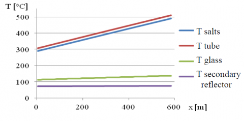
The flow rate $\dot{m}$ set in Table 4 is determined in relation to the velocity of the fluid of 1.35 m/s. For example, for a plant located at a latitude of 39°N, at 12:00 on July 21, the temperatures are shown in Figure 7.
Figure 7. Temperatures obtained for July 21 at 12:00
The temperatures of the fluid and the absorber increase along the direction of motion. The temperature difference between them depends essentially on the value of heat transfer coefficient. The temperature of the glass envelope is maintained at values of about 125 °C, while the secondary reflector is maintained almost at a constant temperature of 70 °C. The temperatures reached by the glass and by the secondary reflector are determined by: their own absorptivity which allows them to absorb part of the solar radiation; the outside air temperature and, above all, the external heat transfer coefficient. In these conditions, the molten salt mixture gets in the plant with a temperature of 290 °C and reaches a temperature of about 497 °C, for a useful thermal power of:
${{P}_{u}}=\dot{m}\,{{c}_{p}}\left( {{T}_{a,out}}-{{T}_{a,in}} \right)\approx 2.5\,MW$ (23)
It may be useful to set the desired outlet temperature and look for the value of the mass flow, at regime, which with different solar irradiation conditions guarantees the outlet temperature predetermined. The procedure consists in varying the flow rate of the salts with a feedback control until the outlet temperature reaches the desired value. In relation to the previous example (July 21, latitude 39° N), by setting the outlet temperature equal to 500 °C the hourly trend of the flow rate of salts which circulate in the system is obtained (Figure 8).
Figure 8. Hourly flow evolving
The integral of the curve of Figure 8 is the quantity of fluid which, in the course of the day, changes its temperature from 290 °C to 500 °C. The result of the integral, in the specific case, is 183,714 kg. Table 5 shows the energy losses (per unit of time) that occur during operation at 12:00 on July 21.
Table 5. Power balance
|
Power balance (kW) |
||
|
Reflected irradiance not incident on tube |
9.9 |
0.31 % |
|
Irradiance absorbed into primary reflectors and lost by convection |
193.4 |
6.00 % |
|
Irradiance absorbed in secondary reflector and lost by convection |
172.3 |
5.36 % |
|
Irradiance absorbed into glass envelope and lost by convection |
57.0 |
1.77 % |
|
Irradiance reflected from steel tube |
166.8 |
5.17 % |
|
Power absorbed by the pipe and lost by irradiance |
128.0 |
3.97 % |
|
Useful power absorbed by the fluid |
2,495.4 |
77.42 % |
|
Total solar irradiance |
3,223.1 |
100 % |
Figure 10 shows, instead, the performance trends as a function of solar irradiation.
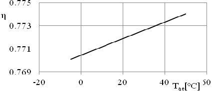
Figure 11 shows graphically the influence of the outside air temperature on total efficiency, which is not very accentuated due to the presence of the glass envelope.
Figure 12, finally, reports the efficiency trend under variable wind speed, which influences the external heat transfer coefficient he on the surface of the glass and, thus, the temperature of the outer tube.
Figure 9. Efficiency against emissivity coating
Figure 10. Efficiency as a function of irradiation
Figure 11. Effects of outside air temperature on the efficiency
Figure 12. Efficiency as a function of wind speed
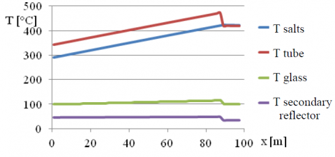
Figure 13 shows the trends of fluid and other components temperatures, carried out for a plant of 100 meters length, with orientation N-S, on 21 December at 12:00.
Figure 13. Temperature trends
In the first length, the temperature of the tube is maintained higher than the fluid, in the second part of the tube it drops rapidly going slightly below that of the fluid, which also reverses its slope. This occurs since the latter part of the absorber (of length k) is not affected by the reflected rays. In this length, in fact, the fluid is cooled as it gives thermal energy to the absorber tube that disperses through radiation to the outside. For this plant, placed at a latitude of 39°N on December 21 at 12:00, according to its geometric characteristics, the length of tube not illuminated k is about 10.4 meters. The yield in the winter solstice, drops down to 65%. The reduction is also due both to the low value of irradiation, which causes the reduction of the flow rate and, then, of the internal heat transfer coefficient and to the low outside air temperature, set equal to 5 °C.
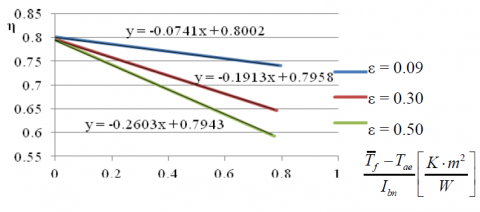
Analysing the results deriving from the simulations, the efficiency curve of the first order is obtained, generally expressed by the following equation:
$\eta=\eta_{o}-a_{1} \frac{\overline{T}_{f}-T_{a e}}{I_{b n}}$ (24)
where:
By performing different simulations, by varying the temperature of the inlet fluid, the outside air temperature and other quantities, it was extrapolated the graph of Figure 14. This graph shows the efficiency curves, in stationary conditions, with reference to different values of emissivity of the surface coating of the receiver tube.
Figure 14. Efficiency curves for different values of emissivity of the coating
3.5 Influence of the plant orientation
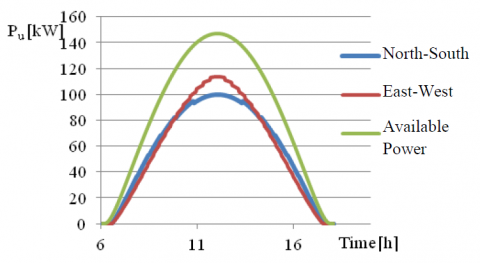
A Linear-Fresnel plant can be disposed according to two types of orientation. It is said that it is oriented in N-S direction if the axis of the tube coincides with the North-South line; it is oriented E-W if the axis coincides with a straight East-West line. In particular, the orientation determines, at various hours of the day, different values of the length of the tube which is not radiated. For small plants this effect has significant influence on the performance. For the plant used in previous simulations but with a length of 30 meters, two graphs that show trends of the absorbed power and efficiencies for both types of orientation, for the Spring equinox, are presented below. Figures 15 and 16 show how the plant with N-S orientation can better direct rays towards the pipe at sunrise and sunset, while the one with E-W orientation directs them better in the middle of the day.
Figure 15. Available power and absorbed power for N-S and E-W plants on March 21
Figure 16. Efficiency for plants N-S and E-W on March 21
Ultimately, to assess which orientation produces more heat energy, it is necessary to solve the integral of the curve of absorbed power. Table 6 presents the values of thermal energy produced in the days of solstices and equinoxes.
Table 6. Produced and available energy, efficiencies
|
March 21 |
June 21 |
September 22 |
December 21 |
|||||
|
N-S |
E-W |
N-S |
E-W |
N-S |
E-W |
N-S |
E-W |
|
|
Eu [MJ] |
2,544 |
2,548 |
3,625 |
3,342 |
2,345 |
2,342 |
922 |
1,080 |
|
Etot [MJ] |
3,717 |
3,717 |
4,877 |
4,877 |
3,448 |
3,448 |
1,588 |
1,588 |
|
ηtot |
0.684 |
0.685 |
0.743 |
0.685 |
0.680 |
0.679 |
0.581 |
0.680 |
${{\eta }_{tot}}=\frac{{{E}_{u}}}{{{E}_{tot}}}$ (25)
In Figure 17 the results obtained for the two orientations for all months of the year are shown in a bar chart. The value of average energy produced daily was estimated and it was found that the collector with North-South orientation is able to provide better performance.
Figure 17. Energy produced the 21th day of month
In this work the performance of a linear Fresnel concentrator was analyzed. A mathematical model was realized, it is based on the finite difference method and allows to determine the temperature profiles of the receiver components and the influence of different parameters on the performance of the plant. It was therefore possible to observe the emissivity of the selective coating that covers the absorber tube has great importance and constitutes the main cause of heat losses.
Thanks to the created model it was also possible to estimate the productive efficiency of the system for the two orientations and for different months of the year. The model created and implemented allows, therefore, at any section of the plant, detection of the temperatures and the powers exchanged between the components, in order to evaluate optical and thermal losses and to identify the parameters on which it is convenient to intervene to increase the efficiency of the same. The simulations show that the system with N-S orientation provides the best performance.
|
||G|| |
matrix of thermal conductance, W.K-1 |
|
|F| |
vector of nodal flows, W |
|
|G| |
vector of nodal temperature, K |
|
a |
solar azimuth, rad |
|
a1 |
thermal losses of collector, W.m-2.K |
|
A |
surface occupied by reflectors, m2 |
|
A1 |
extra-atmospheric apparent solar radiation, W.m-2 |
|
A2 |
atmospheric extinction coefficient |
|
Ac,est |
external area of an element of glass tube, m2 |
|
Ad |
area of an element of secondary reflector, m2 |
|
cp |
specific heat, J.kg-1.K-1 |
|
D |
distance between tube and reflector, m |
|
d |
diameter, m |
|
Etot |
energy available in a day, MJ |
|
Eu |
energy produced in a day, MJ |
|
f |
dimensionless fraction of lighted tube |
|
Fc-d |
view factor between external glass tube and secondary reflector surfaces |
|
h |
height of the tube, m |
|
hi |
internal heat transfer coefficient,W.m-2.K |
|
he |
external heat transfer coefficient, W.m-2.K |
|
Ibn |
direct normal irradiance, W.m-2 |
|
k |
length of tube not irradiated, m |
|
l |
primary reflector width, m |
|
ld |
curvilinear length of secondary reflector, m |
|
lap |
aperture of secondary reflector, m |
|
Lp |
length of the plant, m |
|
$\dot{m}$ |
flow rate, kg.s-1 |
|
n |
number of longitudinal nodes |
|
$\hat{n}$ |
versor normal to primary reflector |
|
$\hat{n}_{S}$ |
sun’s rays versor |
|
$\hat{n}_{t}$ |
reflected beam versor |
|
nRP |
number of primary reflectors |
|
Nu |
Nusselt number |
|
Pr |
Prandtl number |
|
Pu |
useful thermal power, W |
|
$\dot{q}_{r}$ |
solar irradiance incident on mirrors, W |
|
$\dot{q}_{s}$ |
solar irradiance absorbed, W |
|
Ra |
Rayleigh number |
|
Rab |
convective resistance between a and b nodes, K.W-1 |
|
Rcond |
axial conductive resistance, K.W-1 |
|
Re,c |
convective resistance between glass tube and external air, K.W-1 |
|
Re,d |
convective resistance between secondary reflector and external air, K.W-1 |
|
Re |
Reynolds number |
|
Rirr,bc |
Radiative resistance between b and c nodes, K.W-1 |
|
Rirr,cd |
Radiative resistance between c and d nodes, K.W-1 |
|
s |
thickness, m |
|
T |
temperature, °C |
|
Ta,out |
fluid outlet temperature, °C |
|
Tae |
outside air temperature, °C |
|
$\overline{T}_{f}$ |
Average fluid temperature between inlet and outlet, °C |
|
Tin |
inlet temperature, °C |
|
v |
velocity, m.s-1 |
|
Greek symbols |
|
|
α |
absorptivity |
|
ρ |
reflectance |
|
β |
inclination of primary reflector, rad |
|
γ |
Ratio between external diameter of glass tube and aperture of secondary reflector |
|
Δx |
longitudinal distance of nodes, m |
|
ε |
emissivity |
|
η |
plant total efficiency |
|
ηo |
plant optical efficiency |
|
ηtot |
average daily efficiency |
|
λd |
thermal conductivity of aluminum, W.m-1.K |
|
λc |
thermal conductivity of glass Bo-Si, W.m-1.K |
|
λb |
thermal conductivity of steel, W.m-1.K |
|
μ |
dynamic viscosity, kg.m-1.s-1 |
|
σ |
Stephan-Boltzmann constant,W.m-2.K-4 |
|
τ |
transmittance |
|
φ |
solar height, rad |
|
Subscripts |
|
|
a |
molten salts |
|
air |
air |
|
ave |
average |
|
b |
inner tube |
|
c |
glass tube |
|
d |
Secondary reflector |
|
int |
internal |
|
est |
external |
|
RP |
primary reflectors |
|
Apexes |
|
|
i |
longitudinal element |
[1] M. Hannane Regue, T. Benchatti, A. Medjelled, A. Benchatti, “Improving the performances of a solar cylindrical parabolic dual reflection Fresnel miror (experimental part),” International Journal of Heat and Technology, vol. 32, no. 1&2, pp. 171-178, 2014.
[2] K. Zhang, J. Du, X. Liu and H. Zhang, “Molten salt flow and heat transfer in paddle heat exchangers,” International Journal of Heat and Technology, vol. 34, Special issue no. 1, pp. 43-50, 2016. DOI: 10.18280/ijht.34S106.
[3] M. Cucumo, D. Kaliakatsos, V. Marinelli, “General calculation methods for solar trajectories,” Renewable Energy, vol. 11, no. 2, pp. 223-234, 1997.
[4] F. Nicoletti, “Studio del Sistema di Inseguimento per un Impianto Solare a Concentrazione con Riflettore di Fresnel,” M.S. thesis, Dept. DIMEG, Unical, Rende (CS), 2015.
[5] M. Falchetta, A. Gambarotta, I. Vaja, M. Cucumo, C. Manfredi, “Modeling and simulation of the thermo and fluid dynamics of the “Archimede Project” solar power station,” presented at the 19th International Conference on Efficiency, Cost, Optimization, Simulation and Environmental Impact of Energy Systems, ECOS 2006, Aghia Pelagia, Crete, Greece, July 12-14, 2006, pp. 1499-1506.
[6] Valerio Marinelli, Giuseppe Oliveti, Adolfo Sabato, Elementi di Trasmissione del calore, Pitagora Ed., Bologna.
[7] ASHRAE Handbook, Fundamentals, New York, 1989.