OPEN ACCESS
This paper reports a numerical investigation of an atmospheric lean-premixed swirl-stabilized burner. The focus on the flow behavior and flame stability is done at various swirl intensity to better understand the propane turbulent premixed flames. The numerical simulation is carried out using RANS technique with three turbulence closer models Standard k-ε, Realizable k-ε and SST k-ω. This in order to evaluate the performance of these models in the prediction of confined turbulent swirling flows. The turbulence-chemistry interaction scheme is modelled using Finite Rate-Eddy Dissipation model with three step global reaction mechanism. The combustor is operated with air and propane mixture under an atmospheric pressure at a global equivalence ratio of Φ = 0.5. The investigation is done using five different swirl numbers Sn = (0, 0.35, 0.75, 1.05, 1.4), including a validation with the available experimental data. Good agreement is found between RANS results and experimental data, in particular axial and radial velocity profiles, temperature and propane concentration profiles. Results indicate the presence of outer recirculation zone (ORZ) in the inlet burner corner, irrespective of the swirl number. When the swirl number reaches a critical value Sn = 0.75, an inner recirculation zone (IRZ) appears in the center of the burner inlet as a result of vortex-breakdown. Increasing swirl number to an excessive value leads to the propagation of the IRZ upstream the combustion chamber, and consequently the appearance of the flame flashback.
Combustion dynamics, Premixed flame, RANS, Swirl number, Vortex breakdown.
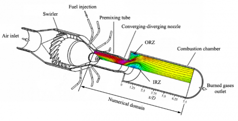
Lean premixed flames (LPMF) are widely used in modern gas turbine combustors. The main advantage of LPMF is the significant reduction in NOx compared to diffusion flames. Most LPMF of gas turbine combustors use upstream a swirler and a sudden expansion in the combustor geometry in order to stabilize the flame. The sudden expansion creates a corner vortex called the outer recirculation zone (ORZ). In addition, the swirler produces a vortex centered on the chamber centerline near the expansion plane. This vortex named inner recirculation zone (IRZ) is known also as a vortex-breakdown phenomenon (Figure 1). The basic concept is that the IRZ serves as an aerodynamic flame holder, which leads to the recirculation of hot burned gases upstream to enhance the ignition of unburned gases and helps to operate the flames under the desired lean conditions. An extensive review on vortex-breakdown and the stability of swirled lean-premixed flames in other burner configurations can be found in [1,2].
Because of the complex turbulent nature of swirling flow phenomena, accurate numerical simulations of such flows require a careful choice of turbulence models. It is generally accepted that the Standard k-ε model [3] can perform reasonably well for simulating simple turbulent flows. Sometimes it provides sufficient results for simulating reacting swirling flows [4] and sometimes it appears inadequate. For example, Sharif et al. [5] reported that the Standard k-ε model shows overestimate the level of turbulent diffusion on a turbulent swirling flow in a cylindrical combustor. It is reported that the deficiency of the Standard k-ε model is due to the use of isotropic eddy viscosity concept, which is not the case for most turbulent swirling flow structures that are anisotropic.
In order to address the deficiency of the Standard k-ε model, Shih et al. [6] purposed the Realizable k-ε model by introducing a new eddy viscosity formula and a new dissipation rate equation. It is based on the dynamic equation of the mean-square vorticity fluctuation at large turbulent Reynolds number. A numerical study using the Realizable k-ε model is presented by AbdelGayed et al. [7] to simulate a premixed high swirl flow in a GT combustor. They found a quite good agreement between the calculated and measured axial and tangential velocities distribution over the whole combustor. They also well captured the IRZ. Recent definition of the turbulent viscosity is proposed by Menter [8] and employed in the shear stress transport (SST) k-ω model, with the addition of a cross diffusion term in the ω-equation. The model shows better performance over the standard k-ε. To investigate the performance of the Standard k-ε and the SST k-ω models, Engdar et al. [9] simulated a confined swirling flow and they found that in a swirling flow with Sn = 0.58, the Standard k-ε model is not able to predict the IRZ, while the SST k-ω model captured this zone.
Regarding the effect of swirl intensity on the flow behavior and the combustion dynamics, numerous studies both experimental and numerical have been conducted. Tsao et al. [10] simulated a can model gas turbine combustor for two swirl numbers (Sn = 0.74 and Sn = 0.85). They found that the swirl momentum is transported to the centerline and formed a vortex core and the strength of this vortex core depends on the inlet swirl levels. Stone et al. [11] studied numerically the impact of three swirl numbers (Sn = 0.56, Sn = 0.84 and Sn = 1.12) on the stability of a lean-premixed gas turbine combustor. For high values of Sn, they observed negative values of centerline axial velocity in the expansion plane which indicating the formation of the vortex-breakdown. Anacleto et al. [12] performed an experimental study of the swirl flow structure and flame characteristics in a lean premixed burner. Their burner contains a swirler with adjustable vanes, which allow using various swirl numbers. They showed that the vortex-breakdown occurs at Sn = 0.5 and IRZ formed at all higher swirl number values. They identify also the flame flashback limit which occurs at Sn = 1.26. Other experimental study was done by Mafra et al. [13] to evaluate the effect of swirl number on the flow and NO emission of LPG cylindrical combustion chamber. The burner was equipped with an adjustable swirl device, allowing to vary the swirl number from Sn =0.36 to Sn = 1.46. As they observed, the fuel-air degree of mixture is mediocre at low swirl numbers and causes the formation of IRZ rich in fuel and it promotes a higher unburned hydrocarbon rate. For higher swirl numbers, a more efficient combustion is observed in IRZ, higher values of temperature, low O2 and NO concentrations. Ying and Vigor [14] investigated the effect of swirling flow on combustion dynamics using Large-Eddy Simulation (LES) technique. They reported that when the swirl number exceeds a critical value Sn = 0.44, vortex-breakdown takes place and leads to the formation of an IRZ. For higher swirl numbers, the turbulence intensity increases, the flame velocity increases which leads to the occurrence of flame flashback. Recently, Martin et al. [15] examined the effect of swirl number on the structure of swirl-stabilized spray flames. They varied the swirl number by changing the swirler configuration, 12 swirl configurations were used. They noticed that the combustion is stabilized and the lifting behavior of the flame depends on the swirl intensity of the flow. More recently, Yilmaz [16] performed numerical study to investigate the effect of swirl number on combustion characteristics in a diffusion flame. He found that the combustion characteristics such as, flame temperature and species concentrations are strongly affected by the swirl number.
The main objective of this paper is to focus on the flow behavior and flame dynamics at various swirl numbers to more clarifying the swirling premixed flames. The flame stability and its limits at each swirl number which is analyzed. A lean premixed swirl stabilized burner experimentally studied by Anacleto et al. [12] is investigated numerically in this study. The approach is based on two dimensional axisymmetric burner geometry, steady state, RANS turbulence models, Finite-Rate/Eddy Dissipation model for chemical reactions and reduced chemical kinetics to three-step schemes for the combustion of premixed propane-air mixture. To treat these objectives, the simulations are done by analyzing the capabilities of three eddy-viscosity turbulence models (Standard k-ε, Realizable k-ε and SST k-ω) in predicting the swirling flow characteristics inside the combustor. Besides, this work attempts to evaluate the performance of Realizable k-ε model which is reported in the literature as the appropriate model to better predict the swirling flows
Firstly, the burner configuration, the computational method and the various numerical modelling are described. Secondly, mesh sensitivity analysis is presented. Thirdly, comparisons between calculations and measurements of detailed profiles of axial and radial velocities, temperature and propane concentration are presented. The experimental data of velocities, temperatures and concentrations were obtained by LDV, thermocouples and sampling probes, respectively. Moreover, in order to illustrate and clarify the effect of swirl intensity the results are presented as follow:
The studied burner configuration is that used by Anacleto et al. [12]. A schematic view of the burner is shown in Figure 1. The model combustor consists of an axial swirl generator, premixing tube (PT), a converging-diverging nozzle and combustion chamber (CC). Because of the sudden expansion downstream of the contraction, a vortex breakdown occurs and the flame is stabilized at the expansion. The swirl generator has a variable blades angle, able to change between 0° and 60° in order to give the flow the desired swirl. The throat diameter D = 40 mm is used to calculate the non-dimensional data presented in the paper. The premixing duct is a cylindrical tube with inner diameter 1.25D and length of 4.14D including the converging-diverging nozzle. The combustion section is a cylindrical tube with inner diameter of 2.75D and total length of 8.4D. As sketched in Figure 1, the model combustor is axisymmetric and the computational domain covers a fraction of the experimental configuration. It includes the premixing tube, the contraction and the combustion chamber. The reference frame is chosen such that x/D is aligned along the symmetry axis and its origin is in the sudden expansion plane (x/D > 0 is the combustion chamber, x/D < 0 is the premixing tube).
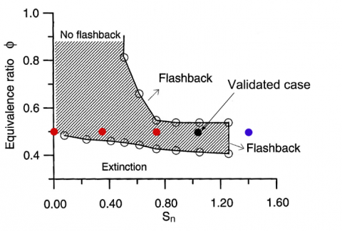
Figure 2 presents the range of combustor operations defined by the flammability and flashback limits, obtained by Anacleto et al. [12]. The leanest and most stable operation condition is found at the global equivalence ratio Φ = 0.5. It is defined as:
Table 1. Summary of Boundary conditions and grid refinement.
|
Procedure |
Case |
Grid |
Total number of cells |
Sn |
w/u |
Turbulence model |
|
Grid convergence |
a |
Coarse |
123 640 |
1.05 |
1.043 |
Realizable k-ε, Standard k-ε and SST k-ω |
|
b |
Medium |
202 380 |
||||
|
c |
Fine |
275 040 |
||||
|
Validation |
1 |
Medium |
202 380 |
1.05 |
1.043 |
Realizable k-ε, Standard k-ε and SST k-ω |
|
Study of swirl effect |
2 |
Medium |
202 380 |
0 |
0 |
Realizable k-ε |
|
3 |
0.35 |
0.347 |
||||
|
4 |
0.75 |
0.744 |
||||
|
5 |
1.4 |
1.39 |
Figure 1. Schematic view of the swirl premixed burner and limits of the numerical domain
$\Phi=\frac{\left(Y_{F} / Y_{O}\right)}{\left(Y_{F} / Y_{O}\right)_{s t}}$ (1)
where YF and YO are respectively the fuel and oxidizer mass fractions. The subscript st indicates stoichiometric conditions (fuel and oxidizer in exact amount so that the combustion is complete).
Inside the burner the flame operates with a perfect mixing of propane and air at atmospheric pressure. The unburned gas temperature at the inlet is Ti = 573 K. Typical averaged velocity at the inlet section of the combustor u0 = 37.7 m/s and the respective diameter are used to calculate the Reynolds number Re = 3.9×10⁴. From the Figure 2, the operating range reduces to a narrow interval of equivalence ratios as the swirl number increases. Therefore, three swirl numbers (red filled circles) are chosen to belong to the stability range of the burner, in addition to the validation case with the experimental data (the black filled circle). One swirl number (blue filled circle) is chosen to be outside the stability range (flashback region). The chosen swirl numbers are equal to 0, 0.35, 0.75, 1.05 and 1.4 corresponding to the swirler blade angels 0°, 22°, 40°, 50° and 58°. The swirl number is defined as the ratio of the axial flux of the tangential momentum to the product of the axial momentum flux and a characteristic radius. The expression of swirl number depends on the injector geometry and flow profiles [17]:
$S_{n}=\frac{\int_{R_{n}}^{R_{h}} \overline{u} \overline{w} r^{2} d r}{\int_{R_{n}}^{R_{h}} R_{n} \overline{u}^{2} r d r}$(2)
where Rn and Rh are the radii of the central body supporting blades and the outer chamber of the swirling device, respectively.
Figure 2. Combustion stability diagram of the burner and studied swirl numbers
Three computational structured grids (coarse, medium and fine) are designed, as presented in Table 1. The difference in these three meshes is mainly due to different grid resolution requirements in order to have a higher resolution in the premixing pipe and in the flame region. To improve near wall grid resolutions a dimensionless wall distance vector y+ = 1 is applied in the three meshes. However, due to the grid influence upon the results the flow has to be solved via a sensitivity analysis using the three grids.
The boundary conditions are summarized in Table 1 and imposed to the geometry as follows: At the beginning of the premixing tube, a mass flow inlet boundary condition is used and a mass flow rate ṁmix = 46 g/s is imposed. Direction vector method in ANSYS-Fluent is chosen, it allows to introduce the three velocity components u, v and w at the inlet of the 2D axisymmetric swirling configuration. A ratio of tangential and axial velocities (w/u) is introduced depending on each swirl configuration, to give the flow the desired tangential (swirling) velocity. A turbulent intensity is introduced also at the inlet and it was estimated from the fully developed pipe flow to be 4.2%. The walls are assumed to be adiabatic and no-slip conditions are also applied. At the outlet the temperature is about 1600 K and pressure outlet boundary condition is applied.
Simulations were performed using the ANSYS-Fluent 16.0 CFD software. It uses the finite-volume method to solve the governing equations. The SIMPLE algorithm is applied for the pressure–velocity coupling. A second order upwind scheme is used for the momentum, turbulence kinetic energy, turbulence dissipation rate, the energy and all species equations. Convergence criteria are set to 10-5 for all equations. The mass and momentum Reynolds-averaged equations are used to solve the turbulent steady flow. As mentioned in the introduction, three turbulence closure models, Standard k-ε, Realizable k-ε and SST k-ω, are used in order to close the system of Reynolds-averaged equations. The detailed description of each model can be found in [3], [6] and [8] respectively.
The hybrid model Finite Rate-Eddy Dissipation plays a key role to address the turbulence-chemistry interaction in the turbulent premixed flames. It is physically based and widely used model which do not demand a high computational effort and offers the use of multi-step reaction mechanisms. The Finite-Rate Kinetics (FRK) model computes the chemical source terms using Arrhenius expressions, and ignores the effects of turbulent fluctuations [18]. A reduced chemical kinetic mechanism of propane-air mixture is employed in the FRK model. This simplified model consists of 3 chemical reactions and 5 species. The three-step scheme of [19] is given below:
$C_{3} H_{8}+3.5 O_{2} \rightarrow 3 C O+4 H_{2} O$
$R_{1}=10^{17.25} \exp (-15106 / T)\left[C_{3} H_{8}\right]^{0.1}\left[O_{2}\right]^{1.65}$(3)
$C O+0.5 O_{2} \rightarrow C O_{2}$
$R_{2}=10^{19.85} e x p(-20142 / T)[C O]^{1}\left[H_{2} O\right]^{0.5}\left[O_{2}\right]^{0.25}$(4)
$C O_{2} \rightarrow C O+0.5 O_{2}$
$R_{3}=5 \times 10^{11} \exp (-20142 / T)\left[C O_{2}\right]^{1}$(5)
5.1 Eddy-dissipation model
Since the used hybrid model includes the Eddy-Dissipation Concept (EDC), a brief description of the model is given. This turbulence-chemistry interaction model is based on the work of [20]. The net rate of production for species i due to reaction r, is given by the smaller of the two expressions below:
$R_{i, r}=v_{i, r} M_{\omega, i} A \rho \frac{\varepsilon}{k} \min \left(\frac{Y_{R}}{v_{R, r} M_{\omega, R}}\right)$(6)
$R_{i, r}=v_{i, r} M_{\omega, i} A B \rho \frac{\varepsilon}{k}\left(\frac{\sum_{P} Y_{P}}{\sum_{j}^{N} v_{j, r} M_{\omega, j}}\right)$(7)
where YR is the mass fraction of a particular reactant R, YP is the mass fraction of any product species P and A, B are empirical constants equal to 4, 0.5 respectively. Finally, after calculating both the Arrhenius and eddy dissipation reaction rates, the Finite Rate-Eddy Dissipation model takes the minimum of these two rates.
5.2 P-1 Radiation model
To obtain a realistic results of temperature it’s necessary to take in account a radiation model during the combustion simulations. The P-1 radiation model [21] is chosen in this study in order to avoid the high computing costs associated with the solution of the radiative transfer equation (RTE).
6.1 Grid sensitivity analysis
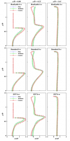
Figure 3. Grid sensitivity solutions of the radial profiles of the axial velocity at several locations with three turbulence models
A grid convergence study is conducted for three meshes shown in Table 1. This analysis is done by simulating the reacting flow using the three turbulence models (Standard k-ε, Realizable k-ε and SST k-ω). A comparison of radial profiles of the mean axial velocity in the combustor is presented in Figure 3. For all models, the profiles of the coarse grid show different tends compared to the profiles of the fine and medium grids. For example, at x/D = 0.22, the coarse grid underestimates the axial velocity near y/D = 1.5, compared to the other grids. In addition, it overestimates the velocity peaks at x/D = 0 and 0.22 for Realizable k-ε and SST k-ω models. The profiles of the fine and the medium grids present exactly the same tends at each location and for each turbulence model. Since the fine grid gives the same results as the medium grid and to reduce the computational efforts, the medium grid is chosen for all calculations in the present study.
6.2 Flow field and temperature distribution
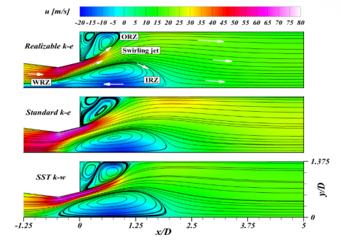
The development of the flow structure over the combustion chamber for the three eddy viscosity models is illustrated in Figure 4, using contours of the axial velocity and the streamline patterns. As expected from a turbulent swirling flow in sudden expansion burner, two distinct regions must be present. The first, a cone-shaped inner recirculation zone (IRZ) appears as a result of the vortex breakdown. This recirculation region is deeply involved in the flame stabilization process, as it constantly puts hot burnt gases in contact with fresh gases allowing permanent ignition. The second, a weak outer recirculation zone (ORZ) comes out above the mixing layer (Swirling jet) and takes its shape from the neighboring boundary walls. Those described characteristics of the flow are captured well by all used eddy-viscosity models. As presented in Figure 4, both models SST k-ω and Standard k-ε show a high velocity gradient in the nozzle throat and the swirling jet region in comparison with Realizable k-ε. This is due to the different definitions of the eddy viscosity that used by each model. Other noticeable zone, a weak recirculation zone (WRZ) upstream the IRZ which appeared in the Realizable k-ε case. It is formed due to the upstream propagation of the IRZ
Figure 4. Predicted axial velocity contours and streamline patterns by the three eddy viscosity models
Figure 5 shows a comparison between the measured and the predicted spatial distribution of temperature along the plane of symmetry in the combustion chamber. The three eddy-viscosity models almost describe the same temperature distribution as the measured data. The IRZ is partially filled with relatively homogenous burned gases, as expected in swirl-stabilized flames, with a maximum temperature of about 1600 K. The ORZ also contributes to flame ignition and stabilization, which is clearly shown in both experimental and numerical results of the present work. Back to the Figure 4 regarding the Realizable k-ε and SST k-ω contours, it is observed that the IRZ extended upstream the expansion plane to reach the throat of the converging-diverging nozzle. This leads to the reduction of the temperature gradient length (black arrows in Figure 5) and make it close to the measured data. The temperature gradient length of the Standard k-ε model reaches a higher value compared to the measured data. This explains the deficiency of the model to predict this kind of complex phenomena caused by a high swirling flow and a fast chemical reaction at the same time.
Figure 5. Comparison between the measured and the predicted spatial distribution of burned gas temperature
6.3 Comparison with experimental data
6.3.1 Axial and radial velocity profiles
Figure 6 shows comparisons between LDA (Laser Doppler Velocimetry) measurements [12], and the present numerical results of axial (a) and radial (b) velocity profiles, at several axial locations in the combustion chamber. The three employed eddy viscosity models can predict the IRZ and the ORZ but with a different accuracy. For example, in Figure 6.a away from the center line ~y/D = 0.54 and at x/D = 0, the measured velocity peak is equal to 1.4u0 and the predicted velocity peaks are: 1.45u0 for Realizable k-ε, 1.7u0 for SST k-ω and 1.9u0 for Standard k-ε model at the radial position ~y/D = 0.62. The Realizable k-ε model predicts the same axial velocity peaks as the measurements in each location. At x/D = 0.22, both Realizable k-ε and SST k-ω models give the same value of the measurements for the centerline axial velocity (y/D = 0). In the locations presented in the Figure 6.b, the three eddy viscosity models produce satisfactory predictions of the radial velocity profiles with a slight difference. The Realizable k-ε is found to be the good model for such kind of flows and it is agreeing with the literature findings. It is chosen for the simulation of the rest of this study.
Figure 6. Eddy viscosity models versus LDA data: radial profiles of the (a) axial and (b) radial velocities
6.3.2 Temperature and propane concentration profiles
A progress variable is used during the validation of the experimental results for both temperature and propane mass fraction. The progress variable of temperature is defined as CT = (T-Tu)/(Tb-Tu), where T is the local temperature, Tu and Tb are the unburned and the burned gas temperatures, respectively. So, if we have CT = 0 it means a fresh gas and if we have CT = 1 it means burnt gas. The progress variable of propane mass fraction Cf is defined with same way as CT.
Figure 7, displays the progress variables profiles of temperature (a) and propane mass fraction (b) in the combustion chamber, predicted by the three eddy viscosity models and compared to the measurements in different locations of the flow. At x/D = 0.25 and ~y/D > 0.7, both Realizable k-ε and SST k-ω models give a good agreement with the experimental results of the progress variables CT and Cf. Around y/D < 0.7 all the eddy viscosity models predict poorly the experimental profiles. A bit far from the expansion plane, beyond x/D = 0.5 and around y/D = 1, the Standard k-ε and SST k-ω profiles are diverge from the measured CT data. Anyway, the Realizable k-ε profile give a good agreement in the same location and also around y/D < 0.7 with measured Cf data., A relatively flat profiles Cf~0 and CT~1 are observed in the far field (x/D ≥ 1.5) for the results of the measurements and the Realizable k-ε model. This indicates that the combustion is nearly finished and no fresh gases are found in this section. The SST k- ω profiles give a poor prediction compared to the measured data in the far field. Once again, the Realizable k-ε proves its capability for predicting the temperature fields at each location.
Figure 7. Eddy viscosity models versus measured data: radial profiles of temperature (a) and propane concentration (b)
6.4 Effect of swirl on flow structures
6.4.1 Velocity distributions
Streamlines along the nozzle and the combustion chamber are plotted for different swirl numbers with axial velocity contours in Figures 8. The first noticeable observation is the presence of the ORZ in the inlet burner corner, irrespective of the swirl number. As the swirl number increases, the length of the ORZ decreases, this is due to the radial expansion of the flow. For example, in the case Sn = 0, the streamlines across the combustion chamber are almost parallel near the centerline. By increasing the swirl number (i.e. Sn = 1.05), the streamlines take the radial direction, as illustrated by the red arrows. The second remark is the formation of the IRZ as the swirl intensity increases. The vortex-breakdown takes place when the swirl number reaches a critical value, this leads to the appearance of the IRZ. In this study, the IRZ appears for three swirl numbers which are Sn = 0.75, 1.05 and 1.4. It can be seen that the length of the IRZ increase with the increase of swirl number. The length of the IRZ reaches 2 x/D for Sn = 0.75, 2.75 |x/D| for Sn =1.05 and 3.75 |x/D| for Sn = 1.4. Note that the values of the IRZ length for Sn = 1.05 and 1.4 are reported using the absolute value, because of the expansion of the IRZ following the negative direction of the x/D axis.
Figure 8. Flow evolution and axial velocity contours for various swirl numbers
6.4.2 Vortex-breakdown identification
At each swirl number, the vortex-breakdown may have identified by plotting the centerline axial velocity along the combustion chamber as illustrated in Figure 9. As can be seen for Sn = 0, the axial velocity along the centerline is positive and it varies between 0.6 and 0.8 u/u0. This confirms the absence of the swirling motion. For Sn = 0.35, by introducing a weak swirling motion the centerline axial velocity decreased in comparison with the previous case to reach 0.25 u/u0 as a minimum value. At Sn = 0.75, the vortex-breakdown appears and negative velocity is identified between 0.13 and 2 x/D. For the higher swirl numbers, the lowest values of the centerline axial velocities are -0.49 u/u0 at 0.74 x/D and -0.83 at 0.55 x/D for Sn = 1.05 and 1.4 respectively.
Figure 9. Centerline axial velocity for various swirl numbers
6.4.3 Swirl velocity evolution.
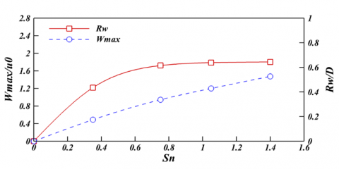
To clarify the discussed issue about the radial expansion of the flow, a parametric study is performed by the determination of the maximum value of the swirl velocity wmax and its corresponding radius Rw, normalized by u0 and D respectively. Figure 10 presents the aerodynamical characteristics of the swirling jet deduced from the swirl velocity and its radial location at x/D = 0.12. It can be seen that the maximum value of swirl velocity wmax increases with increasing of swirl number, as discussed the literature, while Rw the radial location of wmax is shifted outwards confirming the radial expansion of the flow.
Figure 10. Maximum swirl velocity and its radial location at x/D = 0.12
6.5 Effect of swirl on the temperature field
6.5.1 Temperature distribution
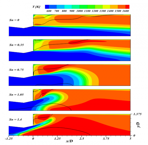
The spatial distribution of temperature for each swirl number is illustrated in Figure 11. The black lines present the iso-value of zero axial velocity in both ORZ and IRZ. For low swirl numbers Sn < 0.35 there is no temperature gradient in the IRZ, only fresh gases are dominated due to the absence of the flow recirculation. But in the ORZ, a high temperature gradient occurs with a maximum value of about 1500 K for Sn = 0 and 1600 K for Sn = 0.35. This is due to the presence of a flow recirculation in this region regardless of the swirl number. This leads to holding the flame and achieve a permanent ignition. By increasing the swirl number, temperature gradient start to fill the IRZ for Sn = 0.75 and it fully locates in the IRZ for Sn = 1.05. For a very high swirl number Sn = 1.4, the temperature gradient appears in the premixing tube and the IRZ almost contains the maximum temperature. This is known as Flashback phenomenon, which is a result of high negative velocity in the IRZ, which leads to the extendibility of its limits to the premixing tube helping to drag the flame inside. These results indicate an optimum range of swirl numbers must be respected to have flame stabilization; above that range an unfavorable flashback phenomenon appears.
6.5.2 Centerline temperature
Figure 12 presents the centerline temperature normalized by the maximum temperature T0 for the different swirl numbers. This allowing to know the length of the reaction zone for each swirl number. With no swirl motion Sn = 0, the centerline temperature is almost constant and takes its lowest value T/ T0 = 0.35, this means there is no reaction in this region. For Sn = 0.35, the combustion at the centerline starts late and the temperature reaches 0.85 of T0 in the outlet of the combustion chamber. For Sn = 0.75, the temperature centerline reaches its maximum value of 0.95 at about x/D = 4.7, this indicate that the reaction zone is near the middle of the combustion chamber. By increasing the swirl number to the optimum value Sn = 1.05, the maximum centerline temperature is achieved early at about 0.97 x/D, and it takes the value of 0.98 T/T0. For a very high swirl number Sn = 1.4, the maximum centerline temperature reaches its maximum value of 1 T/T0 at the combustion chamber inlet, this means that the reaction zone is in the premixing tube which confirms the presence of the flashback in this case.
Figure 11. Spatial temperature distributions for various swirl numbers
Figure 12. Centerline temperature for various swirl numbers
The presented work discusses a numerical simulation of the reacting swirling flow in a lean premixed burner using the ANSYS-Fluent 16.0 software. The results of this work contribute to better understanding the flow behavior and flame dynamics at different swirl intensity, and consequently to define the flame stability limits. Three eddy viscosity turbulent closure models (Standard k-ε, Realizable k-ε and SST k-ω) and the Finite-Rate/Eddy Dissipation model for turbulence-chemistry interaction are used. Those applied approaches are useful to capture the vortex-flame interaction, and the all used models can predict the IRZ and the stabilized flame. Comparing with experimental data, the performance of the eddy-viscosity models in predicting the high swirling flow properties (axial and radial velocities profiles) is competitive. The Realizable k-ε is found to be the good model for such kind of flows and it agrees with the literature findings. It is chosen to simulate the effect of the swirl intensity on the flow structure and flame dynamics in the combustion chamber. Results indicate that for the absence of swirl, the flow is an axial jet and there is no combustion in the inner region of the burner. Whatever the swirl number value, an ORZ appears and holds the flame. At a critical value of the swirl number (Sn = 0.75), an IRZ appears in the center of the burner inlet as a result of the vortex-breakdown. It is found that the length of the IRZ increases with the increase of swirl number. With this increase, the flame tends to stabilize in the inner region of the combustion chamber; consequently, the reaction zone is shortened. At very high swirl number (Sn =1.4), the IRZ expands upstream and downstream the combustion chamber and leads to dragging the flame into the premixing tube. It is found that the swirling flow significantly improves the flame stability, but with increasing the swirl number to an excessive value the flashback appears and the flame is no more stable.
The authors gratefully acknowledge financial support from Algerian Ministry of Higher Education and Scientific Research (PNE 2015-2016).
|
A B Cf CT D k ṁmix Mw,i Re Ri,r Rw Sn T Ti u v w x y+ y YP YR Greek symbols ε Φ ω Subscripts i max mix r |
Empirical constant Empirical constant Progress variable of mean propane Progress variable of mean temperature Diameter of the throat of the nozzle Kinetic energy Mass flow rate of the gas mixture Molar weight of species Reynolds number Reaction rate Radial location of wmax Swirl number Mean Temperature Inlet temperature Mean Axial velocity Mean Radial velocity Mean Swirl or tangential velocity Axial location Wall distance vector Radial location Mass fraction of product Mass fraction of reactant
Turbulent dissipation Equivalence ratio Turbulent frequency
Species Maximum Mixture Reaction |
[1] O. Lucca-Negro and T. O’Doherty, “Vortex breakdown: A review,” Prog. Energy. Combust. Sci, vol. 25, pp. 431-481, 2001. DOI: 10.1016/S0360-1285(00)00022-8.
[2] N. Syred, “A review of instability and oscillation mechanisms in swirl combustion systems,” Prog. Energy. Combust. Sci, vol. 32, pp. 93-161, 2006. DOI: 10.1016/j.pecs.2005.10.002.
[3] B. E. Launder and D. B. Spalding, Lectures in Mathematical Models of Turbulence, London: Academic Press, 1972.
[4] A. Datta and S. K. Som, “Combustion and emission characteristics in a gas turbine combustor at different pressure and swirl conditions,” Appl. Therm. Eng, vol. 19, pp. 949-967, 1999. DOI: 10.1016/S1359-4311(98)00102-1.
[5] M. A. R. Sharif and Y. K. E. Wong, “Evaluation of the performance of three turbulence closure models in the prediction of confined swirling flows,” Comput. Fluids, vol. 24, pp. 81-100, 1995. DOI: 10.1016/0045-7930(94)E0004-H.
[6] T. H. Shih, W. W. Liou, A. Shabbir, Z. Yang and J. Zhu, “A new k-eddy-viscosity model for high Reynolds number turbulent flows,” Comput. Fluids, vol. 24, pp. 227-238, 1995. DOI: 10.1016/0045-7930(94)00032-T.
[7] H. M. AbdelGayed, W. A. Abdelghaffar and K. El Shorbagy, “Main flow characteristics in a lean premixed swirl stabilized gas turbine combustor – Numerical computations,” Am. J. Sci. Ind. Res, vol. 4,
pp. 123-136, 2013. DOI: 10.5251/ajsir.2013.4.1.123.136.
[8] F. R. Menter, “Two-equation eddy-viscosity turbulence models for engineering applications,” AIAA Journal, vol. 32, pp. 1598-1605, 1994. DOI: 10.2514/3.12149.
[9] U. Engdar and J. Klingmann, “Investigation of two-equation turbulence models applied to a confined axis-symmetric swirling flow,” in Proc. Pressure Vessels and Piping Conference, Vancouver, BC, Canada, 2002.
[10] J. M. Tsao and C. A. Lin, “Reynolds stress modelling of jet and swirl interaction inside a gas turbine combustor,” Int. J. Numer. Methods Fluids, vol. 29, pp. 451-464, 1999. DOI: 10.1002/(SICI)1097-0363(19990228)29:4%3C451::AIDFLD796%3E3.3.CO;2-O.
[11] C. Stone and S. Menon, “Swirl control of combustion instabilities in a gas turbine combustor,” Proc. Combust. Inst, vol. 29, pp. 155-160, 2002. DOI: 10.1016/S1540-7489(02)80024-4.
[12] P.M. Anacleto, E.C. Fernandes, M.V. Heitor and S.I. Shtork, “Swirl flow structure and flame characteristics in a model lean premixed combustor,” Combust. Sci. Technol, vol. 175, pp. 1369-1388, 2003. DOI: 10.1080/00102200302354.
[13] M. R. Mafra, F. L. Fassani, E. F. Zanoelo and W. A. Bizzo, “Influence of swirl number and fuel equivalence ratio on NO emission in an experimental LPG-fired chamber,” Appl. Therm. Eng, vol. 30, pp. 928-934, 2010. DOI: 10.1016/j.applthermaleng.2010.01.004.
[14] Y. Huang and V. Yang, “Effect of swirl on combustion dynamics in a lean-premixed swirl-stabilized combustor,” Proc. Combust. Inst, vol. 30, pp. 1775-1782, 2005. DOI: 10.1016/j.proci.2004.08.237.
[15] M. B. Linck and A. K. Gupta, “Twin-fluid atomization and novel lifted swirl-stabilized spray flames,” J. Propul. Power, vol. 25, pp. 344-357, 2009. DOI: dx.doi.org/10.2514/1.35723.
[16] I. Yılmaz, “Effect of swirl number on combustion characteristics in a natural gas diffusion flame,” J. Energ. Resour, vol. 135, pp. 042204, 2013. DOI: 10.1115/1.4024222.
[17] A.K Gupta, D.G Lilley and N. Syred, Swirl flows, London: Abacus Press, 1984.
[18] ANSYS®, Academic Research. Release 16.0. Help System, FLUENT User Guide, ANSYS Inc, 2015.
[19] C. K. Westbrook and F. L. Dryer, “Simplified reaction mechanisms for the oxidation of hydrocarbon fuels in flames,” Combust. Sci. Technol, vol. 27, pp. 31-43, 1981. DOI: 10.1080/00102208108946970.
[20] B. F. Magnussen and B. H. Hjertager, “On mathematical modeling of turbulent combustion with special emphasis on soot formation and combustion,” Proc. Combust. Inst, vol. 16, pp.719-29, 1977. DOI: 10.1016/S0082-0784(77)80366-4.
[21] G. Krishnamoorthy, R. Rawat and P. J. Smith, “Parallelization of the P-1 radiation model,” Numer. Heat Tr. B- Fund, vol. 49, pp. 1-17, 2006. DOI: 10.1080/10407790500344068.