OPEN ACCESS
The reliable geological strength index is the key point of the Hoek-Brown parameters mb, a, s. The geological strength index was created by Hoek, who didn’t give a precise quantitative approach, and based it on structure type and weathering type of rock mass which completely depended on qualitative description and subjective experiences by individuals. The quantitative description of rock structure is achieved by introducing discontinuity volume density of rock masses, whilst, using rock weathering curing degree to quantify the rock type. The discontinuity volume density of rock masses can characterize the distribution of discontinuities in the rock mass and describe occurrence, length, direction, and intensity of discontinuities. Volume density of rock masses and rock weathering curing degree can be quantified accurately by field geological surveys. Then, combining the discontinuity volume density of rock masses and rock weathering curing degree in the general sector scope table, a new quantitative method of GSI is created. Finally, the new method is verified in a rock slope and compared to other methodologies.
Geological strength index; Hoek-Brown criterion, Volume density, Rock weathering degree curing.
In order to guide construction and improve construction programs, it is necessary to update the rock parameters in tunnel and slope engineering. Getting precise mechanical parameters of rock masses can improve work efficiency and create economic benefits. The methods are common in engineering such as the insitu testing method, regular testing method, empirical analysis method, rock mass classification system, and the numerical simulation method [1, 2, 3]. The main disadvantages of in-situ testing are the time requirements, high cost and huge workload, as well as being difficult to implement in rock tunnels and other projects with the results also easily affected by many factors. There is a large error in the results of the regular testing method because of sample interference condition and size. Empirical analysis heavily relies on personal experience. With the numerical simulation method it is difficult to simulate the distribution of the internal structure of the rock. The idea that combines the rock material by preliminary survey work with laboratory experiments is ideal and feasible. Based on this idea, a series of methods such as BQ classification system, RMR classification system, NGI classification system and GSI rock classification system appeared and are used in engineering. The GSI rock classification system based on Hoek-Brown (H-B) strength criterion is the most sophisticated method. The method is based on field investigation and rock tests and produces rock mechanics parameters which give a quantitative output through qualitative input. E. Hoek and E. T. Brown proposed the geological strength index GSI based on the visual impression on rock mass structure and rock weathering assessment. However, the rock structures and rock weathering assessment values quantization process is too rough, so GSI values can’t be accurately obtained. The H–B parameters are difficult to determine and the applicability of jointed rock mass is poor. Therefore, the exact quantification method of GSI is particularly important. So this paper introduces discontinuity volume density of rock masses and weathering curing degree to build a new quantitative analysis method of GSI. The new method was applied in rock slope,with the new GSI quantitative methods analyzed for the precision of the H–B parameter.
E. Hoek and E. T. Brown [4, 5] proposed the H-B strength criterion in 1980. The equations are expressed as follows:
$\sigma_{1}=\sigma_{3}+\sigma_{c}\left(\frac{m_{b}}{\sigma_{c}} \sigma_{3}+1\right)^{0.5}$ (1)
Where σ1 is the maximum principal stresses, σ3 is the minimum principal stresses, σc is the uniaxial compressive strength of the intact rock, mb is the H–B constant of the intact rock.
E. Hoek and E. T. Brown [6] improved the H–B strength criterion in 1992. The equations are expressed as follows:
$\sigma_{1}=\sigma_{3}+\sigma_{c}\left(\frac{m_{b}}{\sigma_{c}} \sigma_{3}+s\right)^{a}$ (2)
Where mb, s and a are the H–B parameters that depend on the degree of fracturing of the rock mass and can be estimated from the RMR [7,8], given by
$m_{b}=m_{i} \exp \left(\frac{R M R-100}{K_{m}}\right)$ (3)
$s=\exp \left(\frac{R M R-100}{K_{s}}\right)$ (4)
$E_{m}=10^{\left(\frac{R M R-10}{40}\right)}$ (5)
This method does not apply when RMR<18,so E. Hoek and E. T. Brown improved the H–B strength criterion and the H–B parameters can be estimated from the Geological Strength Index (GSI) [9,10,11], given by
$m_{b}=m_{i} \exp \left(\frac{G S I-100}{28-14 D}\right)$ (6)
$s=\exp \left(\frac{G S I-100}{9-3 D}\right)$ (7)
$a=\frac{1}{2}+\frac{1}{6}\left(e^{-\frac{G S I}{15}}-e^{-\frac{20}{3}}\right)$ (8)
D is a factor which depends upon the degree of disturbance
to which the rock mass has been subjected by blast damage and stress relaxation. It varies from 0 for undisturbed in situ rock masses to 1 for very disturbed rock masses.
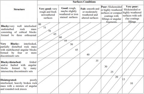
Figure 1 is the method of GSI values given by E. Hoek [10]. The geological strength index GSI is based upon the visual impression on rock mass structure and rock weathering assessment, but the rock structures weathering assessment values quantization process is too rough, preventing accurate GSI values to be obtained. Personal experience of researchers often leads to large deviations. Therefore, the exact value of the GSI is the ruler H–B strength criterion in geotechnical engineering applications, for which, domestic and foreign scholars have done a lot of research. Sonmez et al [12] introduced rock structural hierarchy and rock surface condition rating to achieve a quantitative GSI system. Su Yong-hua et al [13] introduced the rock mass block index and weathering index to depict information of rock mass and realized the quantification of GSI. Cai and Kaiser et al [14] proposed a method for a quantitative GSI system based on block size and joint condition factor JC. Hu Sheng-ming et al [15] proposed a method for a quantitative GSI system based on joint count Jv and joint condition factor JC. These GSI quantitative methods enrich the theory of GSI surrounding rock classification and improve the precision of the GSI value which has great limitations and can not solve the problem of poor application in the joints apparent anisotropy of rocks and a rock’s H–B strength criterion and can’t reflect the influence of rock mass discontinuity on the rock mass strength. The value of GSI can not reflect the characteristics of jointed rock with three-dimensional direction characteristics, and also can not reflect the spatial distribution of rock mass discontinuity which effects the value of GSI.
Figure 1. Geological strength index (GSI) in Hoek-Brown criterion
3.1 Discontinuity areal density
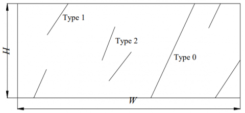
There are a lot of joints, cracks, faults and veins in rock masses that cut the rock mass, leading to the formation of discontinuities. Rock mass is composed of discontinuities and blocks[16]. These discontinuities are randomly distributed while the spatial distribution, spacing, roughness and opening width of discontinuities in rock masses are different. Thus discontinuity areal density and volume density of rock masses obtained from mathematical statistics can be used as important parameters to study the mechanical properties of the rock [17,18]. Figure 1 shows three types of the rock discontinuities in the sample window that: Type 0 doesn’t have a visible endpoint; Type 1 has a visible endpoint; and Type 2 has two visible endpoints.
M. Mauldon [19] defined the average number of discontinuity trace midpoints in the unit area as discontinuity areal density. That does not mean that the discontinuity trace midpoint of Type 0 and Type 1 in the sample window can be obtained. The midpoint corresponds to the exposed upper endpoint and lower endpoint in the sample window. M. Mauldon [19] proposed a method to estimate the number of discontinuity midpoints through the number of discontinuity traces in the sampling window. When the sample window width (W) and height (H) was assumed, the relevant relationship is expressed as follows:
$N=\left(n-n_{0}-n_{2}\right)+2 n_{2}=n-n_{0}+n_{2}$ (9)
Where: n is the number of Type 0 discontinuity traces, n1 is the number of Type 1 discontinuity traces, n2 is the number of Type 2 discontinuity traces, N is the number of discontinuity trace endpoints
$\lambda_{a}=\left(n-n_{0}+n_{2}\right) / 2 W H$ (10)
Figure 2. Sketch of discontinuity traces in sampling window
The equation (9) shows that the number of Type 0 and Type 1 is the number of discontinuity trace endpoints. So, the discontinuity areal density is expressed as follows:
3.2 Discontinuity volume density
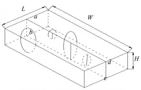
The number of discontinuities at the center of the disk is defined as the discontinuity volume density. In fact, the real situation of rock discontinuities is difficult to obtain by site investigation, only through the relationship between discontinuity volume density with occurrence, length, direction and intensity of the rock discontinuity’s characteristics can an approximate value be obtained. The average vector direction of rock discontinuities and the average diameter of the disk can be obatined by simulating the occurrence of discontinuities and the size of the discontinuities. The approximate value of discontinuity volume density can be calculated by the relationships between the average vector direction of rock discontinuities, the average diameter of the disk and the discontinuity areal density.
Figure 3. Position of Discontinuities center of the disk and the sample window
It should be assumed that the discontinuity center of the disk is evenly distributed in unit volume, and used the average diameter of the disk to replace the size of the discontinuities. Figure 3 shows that the relationship between the total number of discontinuity endpoints with the position of discontinuities in the center of the disk and the sample window abcd. In this case, the discontinuities in the center of the disk associated with the sample window must appear in the range of volume surrounded by the diameter of the disk and the sample window of rock discontinuity.
The discontinuity volume density is expressed by the discontinuity areal density as follows:
$\lambda_{V}=\frac{\lambda_{a}}{D}$ (11)
Where: D is the average diameter of the disk, λV is discontinuity volume density.
The equation (11) shows the relationship between the discontinuity volume density and the discontinuity areal density, but the discontinuity is not necessarily perpendicular to the sample window. It is necessary to correct the sampling window parallel to the normal vector of discontinuities when calculating the volume density. The equation is expressed as follows:
$\lambda_{V}=\frac{\lambda_{a}}{D^{*}}=\frac{\lambda_{a}}{D \sin \gamma}$ (12)
Table 1. Relationship between discontinuity volume density and rock structure
|
discontinuity volume density |
Joints and cracks |
Rock Structure |
|
0~0.35 |
Poor development |
Blocky:very well interlocked undisturbed rock mass consisting of cubical blocks formed by three orthogonal discontinuity sets |
|
0.35~0.50 |
Development |
Very Blocky: interlocked, partially disturbed rock mass with multifaceted angular blocks formed by four or more discontinuity sets |
|
0.50~0.71 |
Good development |
Blocky/disturbed: folded and/or faulted with angular blocks formed by many intersecting discontinuity sets |
|
0.71~0.93 |
Very good development |
Disintegrated: poorly interlocked, heavily broken rock mass with a mixture of angular and rounded rock pieces |
|
0.93~1 |
Completely broken |
Fracture: completely or nearly completely broken |
Where: D* is the normal diameter of the disk, γ is the angle between the vector of discontinuities and the vector of the sample window.
The relevant relationship of the discontinuity volume density is expressed as follows:
$\lambda_{v}=\sum_{j=1}^{m}\left(\lambda_{v}\right)_{j}$ (13)
The relationship between the discontinuity volume density and joints as well as cracks is given in Table1.
3.2 Rock Weathering Curing Degree
Analysis of the microscopic features of rock mass such as the microstructure, micro-fractures, clay mineral and other secondary structures can determine the rock weathering. Table 2 shows that the development of weathering, the secondary infilling of joints and the secondary alteration of feldspar can be used to describe the indicator for determining weathered intensity by Li Riyun and Wu Linfeng [20].
Li Riyun [20] proposed that the grade of alteration mineral, the dispersion degree of the alteration mineral and the percentage of alteration mineral can be used to determine the rock weathering degree curing. The equation is expressed as follows:
$S=\mu \sum_{i=1}^{n} A_{i} * P_{i}$ (14)
Table 2. Indicators for determining weathered intensity
|
Determining weathered intensity |
Microstructure |
Secondary alteration of feldspar |
|
Completely weathered rock |
Disappeared primary structure |
Feldsparsecondary alteration rate more than 95%, disappeared feldspar contours, whole changed toclay mineral |
|
Strong weathered rock |
Blurry primary structure blurry, good development of microcrack |
Feldspar secondary alteration rate of 95% to 70%, feldspar surface completely covered with clay, dust color isn’t bright |
|
Intermediary weathered rock |
Poor clear ignimbrite structure, development of microcrack |
Feldspar secondary alteration rate of 70% to 30%, most of feldspar surface covered with clay, oyster gray isn’t bright |
|
Slightly weathered rock |
Clear ignimbrite structure, Little development of microcrack |
Feldspar secondary alteration rate of 30% to 5%, part of feldspar surface covered with clay, offwhite is bright, fresh feldspar can be seen |
|
Fresh rock |
Very good clear primary structure, disappeared weathered cracks |
Feldspar secondary alteration rate less than 5%, most of feldspar is bright, whole changed toclay mineral, a little of feldspar changed toclay mineral |
Where S is the rock weathering degree curing, μ is the dispersion degree of the alteration mineral, Aiis the grade of alteration mineral, Piis the percentage of alteration mineral. Since the sum of the maximum ratings of these parameters was 20, the value of the ratings for rock weathering curing degree could be calculated and is shown inTable 3.
Table 3. Classification of rock weathering intensity
|
Rock weathering |
Curing degree S |
|
Very good: very rough and fresh unweathered surfaces |
1.00~1.20 |
|
Good: rough, maybe slightly weathered or iron stained surfaces |
1.20~1.40 |
|
Fait: smooth and moderately weathered and altered surfaces |
1.40~1.60 |
|
Poor: Slickensided or highly weathered surfaces or compact coatings with fillings or angular fragments |
1.60~1.80 |
|
Very poor: Slickensided or very weathered surfaces with soft clay coatings fillings |
1.80~2.00 |
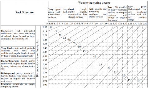
It was the possible to estimate a more precise GSI value from the intersection point of the discontinuity volume density and rock weathering curing degree when the modified GSI chart was used in Figure 4.
Figure 4. Quantificational modification of geological strength index(GSI)
4.1 M-C Transformed into H-B
Since most geotechnical software is still written in terms of the Mohr-Coulomb (M-C) failure criterion, it was necessary to determine equivalent angles of friction and cohesive strengths for each rock mass and stress range. This was done by fitting an average linear relationship to the curve generated by solving Equation (2) for a range of minor principal stress values defined by σt<σ3<σ´3max. The fitting process involved balancing the areas above and below the M-C plot. This resulted in the following equations for the angle of friction φ´ and cohesive strength c´[11]:
$\varphi^{\prime}=\sin ^{-1}\left(\frac{\eta}{2(1+a)(2+a)+\eta}\right)$ (15)
$c^{\prime}=\frac{\eta}{(1+a)(2+a)^{*} \sqrt{1+\eta /(1+a)(2+a)}}$ (16)
$\eta=6 a m_{b}\left(s+m_{b} \sigma_{3 n}^{\prime}\right)^{a-1}$ (17)
$\sigma_{3 n}^{\prime}=\frac{\sigma_{3 \max }^{\prime}}{\sigma_{c i}}$ (18)
It was important to use the appropriate value of σ´3max use in Equations (6) and (7). The fitted equation for the value of σ´3max and the value of σcm is:
$\frac{\sigma_{3 \max }^{\prime}}{\sigma_{c m}}=k\left(\frac{\sigma_{c m}}{\gamma H_{s}}\right)^{m}$ (19)
Where: γ is the unit weight of the rock mass and H is the depth of the tunnel below surface or the height of the slope. The results of the studies for deep tunnels foundnd that k = 0.47 and m =-0.94, and for slopes find that k = 0.72 and m = -0.91. Where: σcm is the rock mass strength, defined by
$\sigma_{c m}=\frac{\sigma_{c i}\left[m_{b}+4 s-a\left(m_{b}-8 s\right)\right]\left(m_{b} / 4+s\right)^{a-1}}{2(1+a)(2+a)}$ (20)
The rock mass modulus of deformation is given by [8]:
$E_{m}=\left(1-\frac{D}{2}\right) \sqrt{\frac{\sigma_{c i}}{100}} * 10^{\frac{G S I-10}{40}}$ (21)
Which is for σci <100MPa and for σci <100MPa [11]:
$E_{m}=\left(1-\frac{D}{2}\right) 10^{\frac{G S I-10}{40}}$ (22)
4.2 Engineering example
A slope builds a bridge located at Guiyang province. The necessary data is collected by authors from this bridge. The slope with a height of 166m and an angle of 36° has a sequence consisting of compact limestone. There are two penetrating joints of the slope which have dip angles with the following parameters: J1: 0°–20°∠80–85°; J2:70°–90°∠80–85°. The rock is cut by two X shaped joints with an angle of 70°. Furthermore, second fault activity had occurred in the region before. Many joints and cracks have developed near the "X" shape and formed many discontinuities of rock masses. The rock of the slope with a uniaxial compressive strength σci of 28 Mpa, has a cohesion c of 600 Kpa, a unit weight γ of 27 KN/m³, an equivalent friction angle φ of 32° and a rock mass modulus Em of 2.08 Gpa.
Figure 5. Simplified CAD drawing of Bridge
The discontinuity volume density of rock mass is computed and the consequent volume density is 0.57. The weathering curing degree is 1.59. The new method used for estimation is shown in Figure 5, obtaining a more precise GSI value of 35. The H–B constant of the intact rock mi is 10. The disturbance factor D is 0. The H–B parameters a, s and mb shown in Table 4 were calculated by the new method.
Table 4. Comparison form of rock mass parameters
|
Method |
GSI |
mb |
a |
s |
σcm |
σ´3max |
φ´ |
c´ |
Em |
|
|
MPa |
MPa |
° |
KPa |
GPa |
||||||
|
|
Rock strength parameters |
|
- |
- |
- |
- |
- |
32 |
600 |
2.08 |
|
1 |
Discontinuity volume density |
35 |
0.9813 |
0.5159 |
0.0007 |
3.48 |
2.87 |
33.1 |
598 |
2.23 |
The discrepancy percentages of φ´, c´ and Em were: 3.44%, -0.034% and 7.21%, respectively. A slope model with a height of 230 m, a width of 310 m, an angle of 36° and the slope height of 170 m was used to analyze the stability with the help of Slope/W module under SIGMA/W in Geostudio 2004. The consequent stability was 1.840. At the same time, the values of the safety factor Fs were 1.844 by the rock strength parameters. It was found that the accuracy of the GSI obtained increased with the increasing capacity for reflecting the distribution of regenerated rock mass discontinuity. The discontinuity volume density and the weathering curing degree can accurately describe the features of rock joints and cracks as well as the degree of fragmentation, degree of disturbance, structural surface filling, and weathering conditions. As the accuracy of the GSI value improved, the discrepancy of the H–B parameters a, s and mb was small. The proposed method solved the problem that the H–B parameters were hard to determine and that their applicability was poor in rock masses with apparent anisotropy characterized by joints and cracks. Thus, our approach can strengthen the practical application of H–B strength criterion, and make it more widely used in geotechnical engineering.
The volume density of discontinuities in rock masses is a function of rock strength as well as the formation of environmental and engineering-geological characteristics. It was found that the discontinuity volume density of rock masses can characterize occurrence, length, direction and intensity of the rock discontinuity characteristics to be studied, and thus it can be used to describe the rock structure. Rock weathering degree curing can be used to describe the development of weathering, the secondary in-filling of joints and the secondary alteration of feldspar.
Based on more precise GSI values obtained from the combination of discontinuity volume density with rock weathering degree curing ratings, a solution can be found to the problem that H–B parameters are difficult to be determined and the applicability is poor in the rock mass with apparent anisotropy characterized by joints and cracks. From comparison of discrepancy percentages with rock strength parameters, the new method utilizing discontinuity volume density with rock weathering degree curing ratings gives the smallest values and produces a better estimation.
The result of the safety factor Fs from the new method utilizing discontinuity volume density with rock weathering degree curing ratings shows that the error is existed in different methods. The value of the safety factor Fs was 1.840 and was smaller than the results of the rock strength parameters at 1.844.
1. YAN Echuan, TANG Huiming, “Stability estimation and utilization of engineering rock mass” [M], Wuhan: China University of Geosciences Press, 2002.
2. A. SADRMOMTAZI, A.K. HAGHI, “Heat Transfer in therophotovoltaics radiation filters” [J], International Journal of Heat and Technology, 2008, 26(1): 59–63.
3. Jianmin Xu, Shuiting Zhou and Kunsheng Li, “Analysis of flow field and pressure loss for fork truck muffler based on the finite volume method” [J], International Journal of Heat and Technology, 2015, 33(3): 85–90. DOI: 10.18280/ijht.330312.
4. HOEK E., BROWN E.T., “Empirical strength criterion for rock masses [J],” Journal of Geotechnical and Geoenvironmental Engineering, ASCE, 1980, 106(9): 1013–1 035. DOI: 10.1016/S1365-1609(03)00025-X.
5. HOEK E., BROWN E.T., Underground Excavations in Rocks [M], London: Institution of Mining and Metallurgy, 1980: 527.
6. HOEK E, WOOD D., SHAH S., “A modified Hoek-Brown criterion for jointed rock masses” [C]// HUDSON J.A. ed., Proceedings of the Rock Characterization, Symposium of ISRM, London: British Geotechnical Society, 1992: 209–214.
7. HOEK E., MARINOS P., BENISSI M., “Applicability of the geological strength index (GSI) classification for very weak and sheared rock masses, the case of the Athens Schist Formation [J],” Bulletin of Engineering Geology and the Environment, 1998, 57(2): 151–160. DOI: 10.1007/s100640050031.
8. HOEK E., BROWN E.T., “The Hoek-Brown criterion — a 1988 update” [C]// CURRAN J.C. ed., Proceedings of the 15th Canada Rock Mechanics Symposium. Toronto: University of Toronto, 1988: 31–38.
9. HOEK E., “Strength of rock and rock masses” [J], International Society for Rock Mechanics News Journal, 1994, 2(2): 4–16.
10. HOEK E., KAISER P.K., BAWDEN W.F., Support of Underground Excavations in Hard Rock [M], Rotterdam: A. A. Balkema, 1995: 99.
11. HOEK E., CARRANZA-TORRES C., CORKUM B., “Hoek-Brown failure criterion—2002 edition” [C]// HAMMAH R., BAWDEN W.F., CURRAN J., et al. ed., Proceedings of the North American Rock Mechanics Society NARMS-TAC 2002, Toronto: University of Toronto Press, 2002: 267–273.
12. SONMEZ H., ULUSAY R., “Modification to the geological strength index (GSI) and their applicability to stability of slopes” [J], International Journal of Rock Mechanics and Mining Sciences, 1999, 36(6): 743–760. DOI: 10.1016/S0148-9062(99)00043-1.
13. SU Yong-hua, FENG Li-zhi, LI Zhi-yong, ZHAO Minghua, “Quantification of elements for geological strength Index Hoek-Brown criterion” [J], Chinese Journal of Rock Mechanics and Engineering, 2009, 28(4): 679–686.
14. CAI M., KAISERA P.K., UNOB H., et al., “Estimation of rock mass deformation modulus and strength of jointed hard rock masses using the GSI system” [J], International Journal of Rock Mechanics & Mining Sciences, 2004, 41: 3-19. DOI: 10.1016/S1365-1609(03)00025-X.
15. HU Sheng-ming, HU Xiu-wen, “Estimation of rock mass parameters based on quantitative GSI system and Hoek-Brown criterion” [J], Rock and Soil Mechanics, 2011, 32(3): 861–866.
16. WANG Liangkui, CHEN Jianping, LU Bo, “Estimation and application of volume density of discontinuities in sampling window” [J], Coal Geology & Exploration, 2002, 30(3): 42-44.
17. ZHOU Fujun, CHEN Jianping, NIU Cencen, “Study of discontinuity density of fractured rock masses based on fractal theory” [J], Chinese Journal of Rock Mechanics and Engineering, 2013, 32(1): 2624-2631.
18. CHEN Jianping, WANG Qing, XIAO Shufang, Computer Simulation Theory of 3D Random Discontinuities Network [M], Changchun: Northeast Normal University Press, 1995: 11-16.
19. MAULDON M., “Intersection probabilities of impersistent joints” [J], International Journal of Rock Mechanics and Mining Sciences and Geomechanics Abstracts, 1994, 31(2): 107–115. DOI: 10.1016/0148-9062(94)92800-2.
20. LI Riyun, WU Linfeng, “Research on characteristic indexes of weathering intensity of rocks” [J], Chinese Journal of Rock Mechanics and Engineering, 2004, 23(22): 3 830-3 834.