Gong Chen* | Lei Cai | Lv Zong | Yan Wang | Xin Yuan
© 2020 IIETA. This article is published by IIETA and is licensed under the CC BY 4.0 license (http://creativecommons.org/licenses/by/4.0/).
OPEN ACCESS
Passive acoustic technology (PAT) is an important tool to acquire the passive acoustic signals from marine organisms. In this paper, PAT fish detection is introduced at great length, including the relevant instruments, signal processing methods, and workflow. Focusing on the key tasks of PAT fish detection, the authors proposed a sparse decomposition algorithm that extracts coherent ratio of passive fish acoustic signal, and designed a feature extraction method for that signal based on speech imitation technology. Experimental results demonstrate that the proposed sparse decomposition algorithm can detect fish acoustic signal accurately at low signal-to-noise ratios (SNRs), and the proposed feature extraction method can effectively extract fish acoustic signals from the marine background. The research results shed important new light on the protection and management of fishery resources in the seas and oceans.
marine organisms, passive acoustic technology (PAT), digital signal processing, feature extraction
The regular surveys on fishery resources are critical to the sustainable development of fishery industry. Acoustic detection methods, both active and passive, provide important tools for such surveys, because fish can squeeze and rub their bladders to produce sound [1]. Active acoustic technology has been successfully adopted to survey the codfish resources in the Yellow Sea, the East China Sea, and the northern Pacific [2].
Passive acoustic technology (PAT) is a non-invasive and non-destructive observation tool that applies the radiation of underwater objects to detection, recognition, and tracking [3]. It can detect and monitor pollutants and organisms in marine environment, which are influenced by human activities. However, PAT has not been widely applied to the survey on fishery resources, due to the following reasons: the sound mechanism of fish is uncertain, the marine environment has complex noises, and few marine biologists are familiar with this technology.
Around the world, over 800 fish species in 109 families are known to be soniferous [4]. Some of them are the most abundant and important commercial fish species, including Gadus morhua, Pseudosciaena polyactis, Oncorhynchus keta, Epinephelus, and Silurus asotus. The earliest application of PAT in fish biology and fishery survey can be dated back to 60 years ago [5]. This technology has been used to determine habitat [6], identify spawning areas [7, 8], and study fish behaviors [9].
Marine ecologists and fishery biologists can listen to the sounds of fish using hydrophones, and process the acoustic signals with digital signal processing algorithms, thereby identifying the fish species [10].
1.1 Passive acoustic source
PAT detects and identifies marine objects by receiving and processing the radiation noise [11]. Captive fish recording and in-situ (natural) recording are two necessary steps of this technology. In captive fish recording, many problems arise from the acoustic complications in a tank or aquarium, combined with the unnatural behavior and sound production. But these problems are not difficult to be overcome.
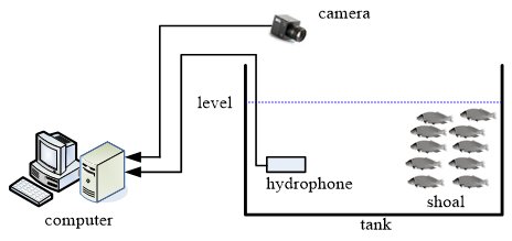
In a particular region, the fish sounds can be catalogued in two ways. The first way is to audition the fish in the field, aquaculture facilities, and public aquaria systematically. The second way is to conduct field surveys to identify the spatiotemporal patterns of sound. Figure 1 illustrates a PAT-based online fish detection system.
Figure 1. The PAT-based online fish detection system
1.2 Collection and recording instruments
Table 1 lists the PAT instruments commonly used to capture the passive acoustic signals from fish. The main detection instruments are hydrophone, hydrophone array, and sonobuoy. The common recording instruments include data recorder, remote sensor, remote control car, and underwater monitoring station. In most recording instruments, high-quality analysis software (e.g. CoolEdit) are embedded to analyze the recorded signals. These instruments have greatly promoted the application of PAT in fishery [5].
1.3 PAT fish detection
The early attempts of fish detection mainly target Sciaenids and Codfishes, which have obvious acoustic features. In the past century, biologists mainly analyzed the reasons, mechanisms, time, and location of fish movements. For instance, Abileah and Lewis [12] introduced the sound surveillance system (SOSUS) of the United States Navy to characterize the salmon spectrum in northern Pacific, and located sound sources with multi-beam and signal processing technologies. Through spectral analysis, Luczkovich et al. [8] identified the sound of Sciaenids through captive fish and natural experiments, and successfully protected the spawning area of the fish. With the aid of hybrid neural network, Howell and Wood [13] differentiated the sound produced by marine organisms from that produced by human activities, and thus identified fish species like Sciaenids and Codfishes. Stolkin et al. [14] detected Codfishes through band-pass filtering and Fourier transform. The above studies show that conventional digital processing technologies are suitable for feature extraction, recognition, and classification of Sciaenids and Codfishes, namely, time-domain filtering, frequency-domain filtering, and neural networks.
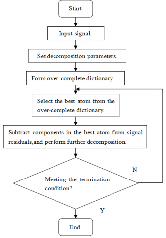
As shown in Figure 2, the PAT fish detection involves data collection, data filtering, endpoint detection, feature extraction, and recognition. Firstly, the passive acoustic signals from the marine environment are collected in captive environment and natural environment. Next, features are extracted from different acoustic signals, forming a feature library. After that, the unknown fish acoustic signals were selected randomly, and compared with the feature library, to identify the fish species.
PAT fish detection needs to deal with five key tasks: (1) build a feature library; (2) disclose the passive acoustic radiation mechanism of marine organisms; (3) identify the feature parameters through digital signal processing; (4) clarify the relationship between sound production and behavior; (5) study the PAT for different species.
Extended from voice activity detection, endpoint detection distinguishes fish sound from noise based on the different features of the same parameters. The distinction relies on the decision criterion called end-point judgement. Through endpoint detection, the denoising effect can be improved by optimizing the feature parameters [15].
One of the most popular sound-noise differentiation algorithms is sparse decomposition, which has been extensively adopted in image processing, video processing, and medical signal processing. Sparse decomposition can decompose the original signal with proper basis functions, without requiring the statistical features of noise. It can also derive the natural features of the original signal from the redundant features in the library. In sparse decomposition algorithm, the coherent ratio reflects the reduction degree of the residual signal compared to the original signal through reconstruction and denoising.
In PAT fish detection, the coherent ratios of fish acoustic signal and noise after sparse decomposition at different signal-to-noise ratios (SNRs) could be extracted to train the detection algorithm. Then, the features of noisy signals can be classified through test. Finally, threshold decision can be adapted to endpoint detection.
2.1 Sparse decomposition
Matching pursuit (MP) algorithm is an adaptive signal decomposition algorithm, which iteratively approximates the local time-frequency structure in a highly redundant complete dictionary with the best matching atom. In PAT fish detection, the low-frequency components of fish acoustic signal are sparse, and similar to the MP atom in structure. But the high-frequency components are stochastic and uncorrelated. The meaningful atoms extracted from fish acoustic signal can demonstrate the distribution of that signal.
Figure 2. The workflow of PAT fish detection
Table 1. The common PAT instruments
|
Name |
Function |
Strength |
Defect |
Application |
|
Hydrophone |
Convert sound pressure into electrical signals. Frequency range: 20Hz-4kHz. Sensitivity: 160-170 dBV/μPa |
Simple to use |
Unable to locate fish distribution |
Widely used |
|
Hydrophone array |
Record data with an array of multiple hydrophones |
Able to locate fish distribution |
In need of complex algorithms |
Partly used |
|
Sonobuoy |
Detect underwater acoustic signals remotely |
Able to detect long-term seasonal fish distribution in a fixed location |
Affected by marine condition; short battery life |
Partly used |
During the iterative sparse decomposition of the signal, the atoms with the biggest inner product between original and residual signals are selected. Through the iterative process, the atomic vectors that best fit the original and residual signals are tracked and extracted constantly, reflecting the distribution of the fish acoustic signal. The coherent ratio serves as the termination condition of the iteration. The Gabor atom in the dictionary can be defined as [16]:
${{g}_{r}}(t)=\frac{1}{\sqrt{s}}g(\frac{t-u}{s})\cos (vt+w)$ (1)
where, $g(t)=e^{-\pi t^{2}}$ is the Gaussian window function; γ=(s,u,v,w) is a set of time-frequency parameters which regulate the expansion, displacement, frequency, and phase position of the atom, respectively.
Figure 3. The workflow of the MP sparse decomposition
As shown in Figure 3, the MP sparse decomposition can be implemented in the following steps:
Step 1. Define the over-complete dictionary $D=\left\{g_{r_{m}}\right\}(m=0,1, \cdots, M-1)$ in Hilbert space, where $\left\|g_{r_{m}}\right\|=1$.
Step 2. Let x(n), n=1,2,…N be the clean acoustic fish signal, where, N is the signal length; x(n)=R0x, n=1,2,…N be the initial residual signal.
Step 3. Select the optimal atom $g_{r_{o}} \in D$ for the MP, and maximize $\left|\left\langle R^{0} x, g_{r_{0}}\right\rangle\right|$, producing the residual $R^{1} x=R^{0} x-\left\langle R^{0} x, g_{r_{0}}\right\rangle g_{r_{0}}$.
Step 4. Select the optimal $g_{r_{1}} \in D$ for the MP, and maximize $\left|\left\langle R^{1} x, g_{r_{1}}\right\rangle\right|$, producing the residual $R^{2} x=R^{1} x-$$\left\langle R^{1} x, g_{r_{1}}\right\rangle g_{r_{!}}, \ldots, R^{m} x=R^{m-1} x-\left\langle R^{m-1} x, g_{r_{m-1}}\right\rangle g_{r_{m-1}}$.
Step 5. Repeat the above steps until the coherent ratio $\lambda\left(R^{m} x\right)=\sup _{g_{r m} \in D} \frac{\left|\left(R^{m} x \cdot g_{r_{m}}\right)\right|}{\left\|R^{m_{x}}\right\|}$ reaches the maximum number M of iterations.
Step 6. Obtain the M+1-st residual $R^{M+1} x=R^{M} x-$$\left\langle R^{M} x, g_{r_{M}}\right\rangle g_{r_{M}}$, $\text { and derive } y(n)=\sum_{m=0}^{M}\left\langle R^{m} x, g_{r_{m}}^{l}\right\rangle g_{r_{m}}^{l}+$$R^{M+1} x, n=1,2, \ldots N$.
Step 7. Select the coherent ratio for the parameters of fish acoustic signal.
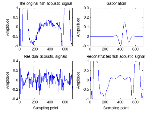
Figure 4 presents the sparse decomposition of passive acoustic signal emitted by Campylomormyrus elephas. It can be seen that the original acoustic signal covered the periodic high amplitude pulse and trailing signal.
Figure 4. The sparse decomposition of passive acoustic signal of Campylomormyrus elephas
2.2 Result analysis
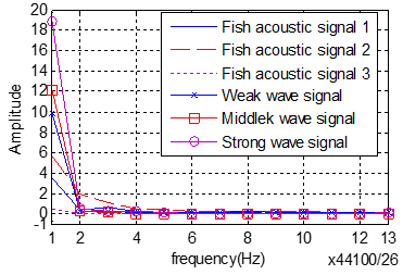
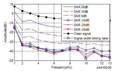
Three groups of clean passive acoustic signals of Campylomormyrus elephas and three groups of wave passive acoustic signals were sampled at a frequency of 44.1kHz, and subject to detection by sparse decomposition, power amplitude and power spectrum methods (in the order of 26). Each clean fish acoustic signal was added strong wave noises at different SNRs. Figure 5 show the coherent ratio, power, and power spectrum distributions at different SNRs.
As shown in Figure 6(a), the fish acoustic signals were similar in amplitude and trend, with obvious difference from the wave signals. The passive acoustic signals of the fish exhibited strong nonstationary, and marked low-frequency features. By contrast, the wave noises exhibited good stability, and unobvious low-frequency features.
During sparse decomposition, the atomic signal was initially easy to match with the low-frequency signal of fish acoustic signal, but difficult to match the wave noise of high frequency. Hence, the residual signal of fish acoustic signal was lower than wave signal. In addition, the nonstationary fish acoustic signal made wave signal more volatile.
As shown in Figure 6(b), fish acoustic signal and wave signal had some individual differences in the low-frequency band. Apart from these, the two signals almost coincided with each other in most frequencies. There were less significant differences compared to the eigenvalue of coherent ratio. Compared to Figure 6(a), Figure 6(b) presents obvious difference in individual distribution. But the fish acoustic signal and wave signal did not have significant differences.
(a) Coherent ratio
(b) Power
(c) Power spectrum
Figure 5. The coherent ratio, power, and power spectrum distributions at different SNRs
It can be further inferred from Figure 6(a) that the distribution of the coherent ratio was close to the fish acoustic signal, when the SNR was greater than 0dB. The distribution was still close to that signal, when SNR dropped to -10dB. As the SNR gradually fell to -20dB, the distribution slowly approximated the wave signal. The approximation to the wave signal was not obvious. To sum up, the gradual decrease of SNR makes the distribution of the coherent ratio approach the strong wave noise.
In conclusion, even if fish acoustic signal is hidden in wave signal, it can be discriminated accurately when the SNR is within -10dB. Hence, the coherent ratio can be used to characterize different acoustic signals. The difference in coherent ratio facilitates the endpoint detection of passive fish acoustic signal.
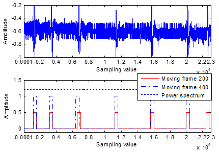
Figure 7 displays the time-domain waveforms and endpoint detections results of passive acoustic signal of Gnathonemus petersii at different low SNRs.
(a) Coherent ratio
(b) Power spectrum
Figure 6. The fish acoustic signals at different SNRs
(a) Clean acoustic signal and detection results based on power spectrum at SNRs of 10, 20, and 30dB (frameshift: 400 points)
(b) Time-domain waveform and endpoint detection result at SNR of 0dB
(c) Time-domain waveform and endpoint detection result at SNR of -10dB
Figure 7. The time-domain waveforms and endpoint detections result of passive acoustic signal of Gnathonemus petersii at different low SNRs
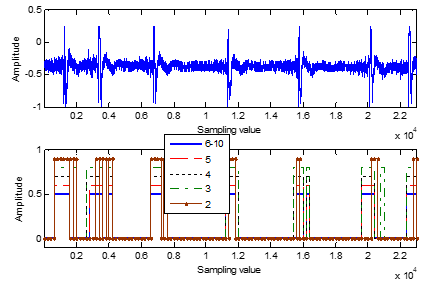
(a) 0dB
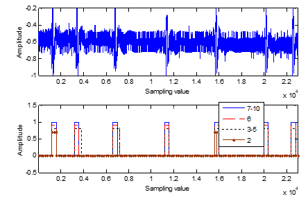
(b) -10dB
Figure 8. The different endpoints of sparse decomposition of the passive acoustic signal of Gnathonemus petersii
As shown in Figure 7, the accuracy of endpoint detection improved, as the SNR increased from 10dB to 30dB based on the features of the power spectrum. When the SNR was below 20dB, it was impossible to detect fish acoustic signal effectively. As the frameshift reached 400 and 200 samples, the signal could be distinguished from noise by coherent ratio. Overall, the sparse decomposition algorithm could differentiate the endpoints of acoustic signal from those of wave noise accurately, when the SNR reached -10dB; the accuracy of 200 frames was better than that of 400 frames.
In fact, fish acoustic signal and wave noise have tiny difference in power spectrum (Figures 5(a) and 6(b)). When the SNR was below 0dB, the signal spectrum was close to the wave noise spectrum. As can be seen in Figure 7, the fish acoustic signal could not be detected by power spectrum method. Under the SNR of 0dB and -10dB, better degree of discrimination ensures a relatively high accuracy of detection.
As shown in Figure 8(a), the signal tail and noise were similar in time-domain amplitude, when the SNR was 0dB. But the frequency of the tail part was lower than that of noise. In this case, the sparse decomposition algorithm will judge the tail signal as fish acoustic signal.
When the SNR was -10dB, the fish acoustic signal was not detectable, for the tail was submerged in the noise at a low SNR. However, the detection accuracy increased with the reduction of frameshift: the detection accuracy was higher at the frameshift of 200 than at that of 400.
It can also be seen from Figure 8 that the detection effect improved in the presence of six features at SNR=0dB, and in the presence of seven features at SNR=-10dB. Hence, the detection efficiency can be improved by reducing the features.
In summary, this section extracts the coherent ratio through sparse decomposition. First, the sparse decomposition algorithm mines the eigenvalues of clean passive fish acoustic signal and wave noise at different SNRs through training, and treat them as the target features in acoustic test. Then, moving noise segment and the target features were extracted for classification in the detection stage. Finally, threshold decision was adapted to detect the endpoints. The experimental results show that sparse decomposition algorithm can detect the fish acoustic signal more accurately than power spectrum method at low SNRs.
The feature extraction technologies mainly focus on time- and frequency-domain analyses. Lobel and Mann [17] obtained weak acoustic signal form damselfish through signal processing. Sprague et al. [18] identified drum fish in captive and natural environments by spectral analysis. To recognize fish species, Wood et al. [19] collected radiated fish signal with hydrophone, and conducted signal processing and spectrum analysis. Using hybrid neural network, Howell and Wood [20] differentiated between marine animal sound, the sound produced by human activities, and the sound of geological source. Stolkin et al. [21] obtained features of codfish through band-pass filtering and fast Fourier transform (FFT). Ren et al. [22] and Liu et al. [23] summarized the sounding principle and signal features of large yellow croaker. Overall, few scholars have adapted them to the noisy environment in seas and oceans. With the help of speech imitation technology, this section extracts effective features from the passive fish acoustic signal.
3.1 Feature parameters
The passive fish acoustic signal has several feature parameters: time-domain feature parameters, and spectral feature parameters. The former parameters are simple, real-time, and easy to classify, but susceptible to noise pollution; the latter are important features in the frequency domain. The frequency-domain features contribute more to denoising than time-domain features. Inspired by speech imitation technology, speech feature parameters [24] were adopted for feature extraction from the passive fish acoustic signal.
(1) Linear prediction coefficient (LPC) and derivative parameters (e.g. LPC cepstrum, and transfer LPC cepstrum)
The time-domain acoustic targets can be described by an autoregressive (AR) model:
$x(n)=\xi (n)-\sum\limits_{i=1}^{p}{{{a}_{i}}}x(n-i)$ (2)
where, ai is the LPC; p is the order of the AR model; ξ(n) is input excitation.
In essence, the LPC analysis searches for the optimal fit to the envelope of the acoustic spectrum from a given sequence of target signals. The AR acoustic spectrum can be estimated by:
$R(t)={\sigma _{\xi }^{2}\Delta t}/{\left| 1+\sum\limits_{i=1}^{p}{{{a}_{i}}\exp (-j2\pi fi\Delta t)} \right|}\;$ (3)
where, $\Delta t$ is the sampling interval; $\sigma_{\xi}^{2}$ is the variance of excitation. The AR spectrum is a high-resolution method for power spectrum estimation. The power spectrum reflects the energy of acoustic signal along with frequency distribution. Formula (3) shows that AR spectrum is closely correlated with the LPC, suggesting that the LPC can reasonably extract features from acoustic signals.
(2) Speech spectrum parameters
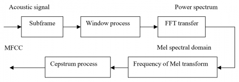
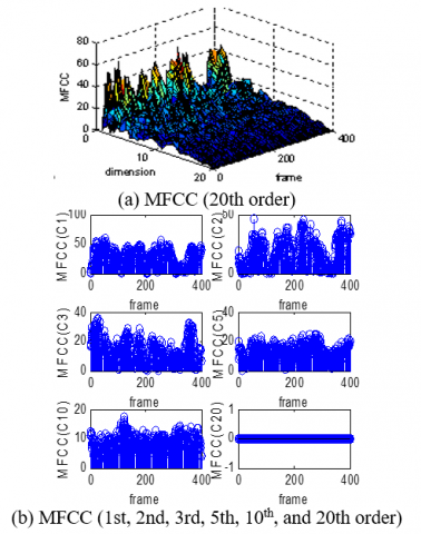
Mel frequency cepstral coefficient (MFCC) simulates the auditory process of speech. It is affected by the performance of the human auditory system. This parameter boasts a strong recognition effect, because the ears can accurately capture the sound amplitude with its ability to detect nonlinear psychological frequency. Figure 9 shows the workflow of MFCC feature extraction.
Figure 9. The workflow of MFCC feature extraction
Fish acoustic signal and speech signal, both originate in medium vibration, carry similar acoustic features. The fish makes sound with bladder, while the speech is produced by the vibration of the vocal cord. The amplitude of speech signal is the mean sound intensity in a short time. It is generally below 90dB. The signal of each word occupies several short time segments. Thus, the mean amplitude of multiple word signals equals the amplitude of the speech signal. The relationship between mean amplitude of passive fish acoustic signal and the amplitude of fish sound is similar.
The short-time zero crossing rate of speech signal refers to the number of zero crossing axes in a given time. This rate of fish sound reflects the frequency of the acoustic target. By likening the fish sound to speech, it is possible to extract the features of passive fish acoustic signal by speech imitation technology.
3.2 Result analysis
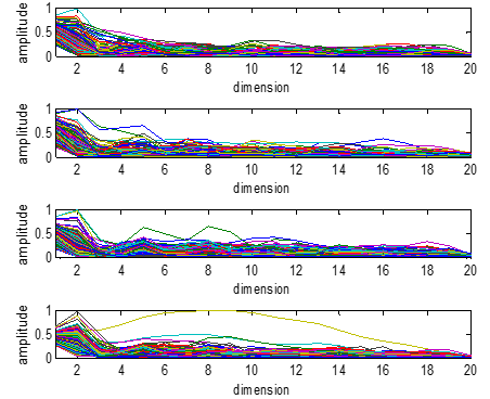
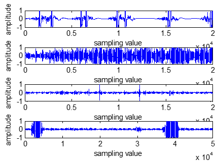
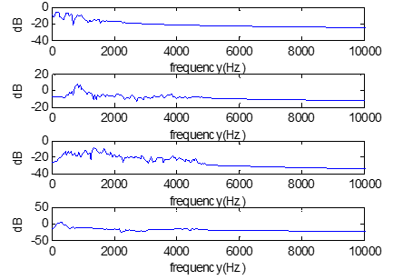
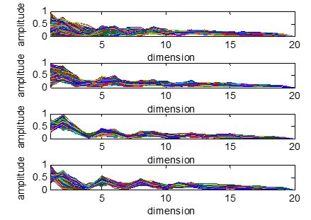
The passive acoustic signals of different fish species were selected from a database. Figure 10 presents the acoustic features of Longnosed Elephant fish, Gnathonemus petersii, Marcusenius cyprinoids, and Brienomyrus brachyistius.
(a) Time domain
(b) Frequency domain
(c) LPC coefficient
(d) MFCC coefficient
Figure 10. The acoustic features of Longnosed Elephant fish, Gnathonemus petersii, Marcusenius cyprinoids, and Brienomyrus brachyistius
As shown in Figure 10, the four acoustic signals all had pulse waveforms; the frequencies of the four signals fell between 100 and 5,000Hz, and peaked at 258, 172, 30, and 87Hz, respectively; only a dozen of LPC dimensions could describe the signal features of acoustic target satisfactorily; the LPC coefficient had a poor performance in feature description, despite its low complexity and limited computing load; the MFCC coefficient had a better performance than the LPC coefficient.
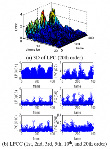
Figure 11. The acoustic signal and LPC parameters
Figure 11 is a three-dimensional (3D) figure of LPC parameters extracted from the acoustic signals of Longnosed Elephant fish in natural environment at the frameshift of 20ms. Specifically, the 20-th order LPC parameters are presented in Figure 11(a), and the 1st, 2nd, 3rd, 5th, 10th, and 20th order LPC parameters are given in Figure 11(b). It can be seen that the first-order component reflected the energy of the acoustic signal higher than other components. With the growing order, the LPC parameter of each component of the amplitude decreased. When the order reached a dozen, the mean amplitude was about 1/10 of the first and second components. Because of small value, its contribution to the feature extraction effect is relatively small.
Figure 12 is a 3D figure of MFCC parameters extracted from the acoustic signals of Longnosed Elephant fish in natural environment at the frameshift of 20ms. Specifically, the 20-th order MFCC parameters are presented in Figure 12(a), and the 1st, 2nd, 3rd, 5th, 10th, and 20th order MFCC parameters are given in Figure 12(b). Comparing Figures 11 and 12, MFCC parameters were more efficient than LPC parameters, in spite of their higher computing load.
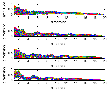
As shown in Figure 13, the acoustic signals of Longnosed Elephant fish, Mosquito fish, Abudefduf saxatilis, and Piranha in natural environment were composed of pulse and non-stationary signals. These acoustic signals fell in the frequency range of 100-5,000Hz, and peaked at 258, 861, 1,723, and 344Hz, respectively.
The LPC difference among different fish species was greater than that of the same fish specie in Figure 10. In addition, the MFCC difference was more discriminative than the LPC difference, and more robust than the MFCC difference of the same fish specie in Figure 10.
In summary, this section proposes a feature extraction method for passive fish acoustic signal based on speech imitation technology. Based on the similarity between passive fish acoustic signal and speech mechanism, this feature extraction method can effectively extract fish acoustic signals from the marine background. Experimental results confirm that the parameters of this method have few feature dimensions, boast strong robustness, and require small calculation. The proposed method shed new light on the protection of fishery resources.
Figure 12. The acoustic signal and MFCC parameters
(a) Time domain
(b) Frequency domain
(c) LPC coefficient
(d) MFCC coefficient
Figure 13. The different features of the Longnosed Elephant fish, Mosquito fish, Abudefduf saxatilis, and Piranha
As a novel marine engineering technology, the PAT attracts much attention from scholars at home and abroad. After a detailed introduction to the PAT, this paper designs a sparse decomposition algorithm and a feature extraction method for fish acoustic signal in marine environment, and verifies the effectiveness of the proposed methods through experiments. The proposed methods solve the key tasks in the PAT fish detection, and help to detect the habitat and living habits of fish and other marine organisms. With the development of the PAT, the proposed methods have great prospects in marine fishery.
This work is supported by Key Laboratory of Nondestructive Testing (Nanchang Hangkong University), Ministry of Education; Collaborative Innovation Center for Cultural Creativity of Colleges and Universities in Jiangsu Province, China (Grant No.: XYN1805); Excellent Science and Technology Innovation Team of Colleges and Universities in Jiangsu Province, China.
[1] Keren, Y. (1994). Underwater sound on fish. Navigation. 12-13.
[2] Tang, Q.S., Wang, W.Y., Chen, Y.Z., Li, F.G., Jin, X.S., Zhao, X.Y., Chen, J.F., Dai, F.Q. (1995). Investigation on the evaluation of the North Pacific Pollock Resources acoustics. Journal of Fisheries of China, 19(1): 8-20.
[3] Tian, T., Liu, G.Z., Sun, D.J. (2000). Sonar Technology. Haerbing: Harbin Engineering University, 1-26.
[4] Lagardere, J.P., Mallekh, R., Mariani, A. (2004). Acoustic characteristics of two feeding modes used by brown trout (Salmo trutta), rainbow trout (Oncorhynchus mykiss) and turbot (Scophthalmus maximus). Aquaculture, 240(1-4): 607-616. https://doi.org/10.1016/j.aquaculture.2004.01.033
[5] Connaughton, M.A., Taylor, M.H. (1995). Seasonal and daily cycles in sound production associated with spawning in the weakfish, Cynoscion regalis. Environmental Biology of Fishes, 42(3): 233-240. https://doi.org/10.1007/BF00004916
[6] Rountree, R.A., Gilmore, R.G., Goudey, C.A., Hawkins, A.D., Luczkovich, J.J., Mann, D.A. (2006). Listening to fish: applications of passive acoustics to fisheries science. Fisheries, 31(9): 433-446. https://doi.org/10.1577/1548-8446(2006)31[433:LTF]2.0.CO;2
[7] Mallekh, R., Lagardere, J.P., Eneau, J.P., Cloutour, C. (2003). An acoustic detector of turbot feeding activity. Aquaculture, 221(1-4): 481-489. https://doi.org/10.1016/S0044-8486(03)00074-7
[8] Luczkovich, J.J., Sprague, M.W., Johnson, S.E., Pullinger, R.C. (1999). Delimiting spawning areas of weakfish Cynoscion regalis (family Sciaenidae) in Pamlico Sound, North Carolina using passive hydroacoustic surveys. Bioacoustics, 10(2-3): 143-160. https://doi.org/10.1080/09524622.1999.9753427
[9] Chen, G., Wang, P.B., Bao, Y.J., Xu, Q.Q., Yang, H., Chen, Z.T. (2016). Research on the detection of weak transient passive fish acoustic signals based on Hilbert–Huang Transform. Marine Sciences, 40(10): 91-96.
[10] Xu, F., Zhang, Q., Zhang, C., Su, R.W. (2015). Walsh transform for fish identification. Applied Acoustics, 34(5): 465-470.
[11] Chen, J.J., Lu, J.R. (2004). A review of techniques for detection of line-spectrum in passive sonar. Shengxue Jishu, 23(1): 57-60.
[12] Abileah, R., Lewis, D. (1996). Monitoring high-seas fisheries with long-range passive acoustic sensors. In OCEANS 96 MTS/IEEE Conference Proceedings. The Coastal Ocean-Prospects for the 21st Century, 1: 378-382. https://doi.org/10.1109/OCEANS.1996.572776
[13] Howell, B.P., Wood, S. (2003). Passive sonar recognition and analysis using hybrid neural networks. In Oceans 2003. Celebrating the Past. Teaming Toward the Future, 4: 1917-1924. https://doi.org/10.1109/OCEANS.2003.178182
[14] Stolkin, R., Radhakrishnan, S., Sutin, A., Rountree, R. (2007). Passive acoustic detection of modulated underwater sounds from biological and anthropogenic sources. In OCEANS 2007, 1-8. https://doi.org/10.1109/OCEANS.2007.4449200
[15] Han, L.H., Wang, B., Duan, S.F. (2010). Development of voice activity detection technology. Application Research of Computers, 4: 1220-1226.
[16] Wang, J.Y., Yin, Z.K., Zhang, C.M. (2006). Sparse Decomposition and Preliminary Application of Signals and Images. Chengdu: Xian Jiao Tong University Press. 1-191.
[17] Lobel, P.S., Mann, D.A. (1995). Spawning sounds of the damselfish, Dascyllus albisella (Pomacentridae), and relationship to male size. Bioacoustics, 6(3): 187-198. https://doi.org/10.1080/09524622.1995.9753289
[18] Sprague, M.W., Luczkovich, J.J., Pullinger, R.C., Johnson, S.E., Jenkins, T., Daniel III, H.J. (2000). Using spectral analysis to identify drumming sounds of some North Carolina fishes in the family Sciaenidae. Journal of the Elisha Mitchell Scientific Society, 116(2): 124-145. https://www.jstor.org/stable/24335502
[19] Wood, M., Casaretto, L., Horgan, G., Hawkins, A.D. (2002). Discriminating between fish sounds—a wavelet approach. Bioacoustics, 12(2-3): 337-339. https://doi.org/10.1080/09524622.2002.9753741
[20] Howell, B.P., Wood, S. (2003). Passive sonar recognition and analysis using hybrid neural networks. In Oceans 2003. Celebrating the Past... Teaming Toward the Future (IEEE Cat. No. 03CH37492), 4: 1917-1924. https://doi.org/10.1109/OCEANS.2003.178182
[21] Stolkin, R., Radhakrishnan, S., Sutin, A., Rountree, R. (2007). Passive acoustic detection of modulated underwater sounds from biological and anthropogenic sources. In OCEANS 2007, Vancouver, BC, Canada, pp. 1-8. https://doi.org/10.1109/OCEANS.2007.4449200
[22] Ren, X.M., Gao, D.Z., Yao, Y.L., Yang, F., Liu, J.F., Xie, F.J. (2007). Occurrence and characteristic of sound in large yellow croaker (Pseudosciaena crocea). Journal of Dalian Fisheries University, 22(2): 123-128.
[23] Liu, Z.W., Xu, X.M., Qin, L.H. (2010). Sound characteristics of the large yellow croaker, Pseudosciaena crocea (Sciaenidae). Technical Acoustics, 29: 342-343.
[24] Han, J.Q. (2019). Voice Signal Processing, Beijing: Tsinghua University Press.