Qi Qi | Shengbang Song*
© 2020 IIETA. This article is published by IIETA and is licensed under the CC BY 4.0 license (http://creativecommons.org/licenses/by/4.0/).
OPEN ACCESS
The governance of industrial water environment in the Yangtze River Economic Belt (YREB), the demonstration zone of ecological civilization in China, has attracted a growing attention. In this paper, an evaluation index system (EIS) with undesired output is established for industrial water resource utilization efficiency (IWRUE). Next, the stochastic block model (SBM) was adopted to measure the IWRUEs of the 11 YREB provinces in 2003-2017. After that, the Tobit model was employed to examine the influencing factors of the IWRUE. The results show that the YREB provinces differed sharply in IWRUE through the sample period; the downstream provinces achieved relatively satisfactorily IWRUEs, while most provinces in the upstream and midstream performed unsatisfactorily. The downstream of the YREB realized the highest IWRUE, followed in turn by the upstream, and the midstream. The YREB is significantly promoted by economic development, ownership structure, and opening-up, and significantly suppressed by water endowment, technological progress, and government influence.
Yangtze River Economic Belt (YREB), industrial water resource utilization efficiency (IWRUE), influencing factors, stochastic block model (SBM), Tobit model
The Yangtze River Economic Belt (YREB) includes 11 provincial administrative regions (hereinafter referred to as provinces), namely, Shanghai, Jiangsu, Zhejiang, Anhui, Jiangxi, Hubei, Hunan, Chongqing, Sichuan, Yunnan, and Guizhou. The 2.05 million km2 region boasts more than 40% of China’s population, and produces over 2/5 of the national gross domestic product (GDP). The YREB towers over any other region in China in terms of comprehensive strength and strategic support.
Nevertheless, the long-term intense economic development has brought severe water shortage and water pollution in the YREB. In particular, the industrial sector, as the second largest water consumer after agriculture, maintains an extensive water use pattern. The amount of industrial water use increases year by year, but the efficiency of industrial water use remains low. In 2017, the YREB consumed 81.54 billion m3 of industrial water, up by 21.88% from the 66.9 billion m3 in 2003.
To make matters worse, a large amount of industrial wastewater is directly discharged into the Yangtze River, due to the lack of effective supervision. The wastewater far exceeds the self-purification capacity of the water body, and strains the environmental carrying capacity of the water environment in the river. Currently, the chemical oxygen demand (COD), ammonia nitrogen (NH4+-N), nitrogen oxides (NOX), and volatile organic compounds emission intensity per unit area in the YERB are 1.5 to 2.0 times the national average. In this context, the only way to realize the sustainable development of YREB water environment is the improve the industrial water resource utilization efficiency (IWRUE).
The IWRUE has long been a hot topic among researchers. For example, Alnouri et al. [1] identified the problems in the current industrial water use pattern, such as heavy water consumption, serious water pollution, and high treatment cost, highlighting the need to evaluate IWRUE. Earlier, Filippini et al. [2] measured the IWRUE of Slovenia through stochastic frontier analysis (SFA). Later, Wang et al. [3] adopted the stochastic block model (SBM) to evaluate the IWRUEs of 30 Chinese provinces in 2009 and 2010. Through dynamic data envelopment analysis (DEA), Pointon and Matthews [4] assessed the efficiency of the wastewater treatment industry in England and Wales. All of the above studies have found that IWRUE has not been optimized, and should be further improved.
On IWRUE improvement, Mortier et al. [5] studied industrial water management in steelmaking industry, laying the basis for sustainable use and management of water resources. From the angles of economy, society and policy, Krause [6] explored the measures and strategies for industrial water saving. In addition, Deason et al. [7] investigated the efficient use of industrial water resources by reforming the water resource system.
To sum up, quite a few results have been accumulated on the IWRUE. However, there are two defects with the existing studies: First, many scholars have examined the IWRUE in different countries, but few have tackled the IWRUE in the YREB. Second, the evaluation index systems (EISs) of the IWRUE rarely contain the pollutants generated in the utilization of industrial water resources. The neglection of the pollutants goes against the reality, resulting in errors in the evaluated IWRUE.
To overcome the defects, this paper establishes an IWRUE EIS containing undesired output (industrial COD), and measures the YREB IWRUE with the SBM. On this basis, the factors affecting the YREB IWRUE were discussed in details. The research results provide a reference for solving the problems in the industrial water environment of the YREB.
2.1 SBM
The traditional research on the IWRUE emphasizes the good outputs over the bad outputs (e.g. water pollutants) of the utilization of industrial water resources. The bad outputs can be regarded as the environmental cost incurred in the utilization process. Nanere et al. [8] held that the neglection of bad outputs might bias the evaluated efficiency. How to implement efficiency evaluation with bad outputs has been well studied over the years.
In efficiency evaluation, traditional approaches like Chames-Cooper-Rhodes (CCR) model and Banker-Chames-Cooper (BCC) model can only handle good outputs. If the efficiency evaluation involves bad outputs, the common practice either treats these outputs as inputs [9], or takes the reciprocals of the outputs as good inputs [10].
None of the above treatments are in line with the actual production activities, and bound to cause errors in the evaluated efficiency. The problem of efficiency evaluation with bad outputs was not solved perfectly until the SBM was proposed by Tone [11]. The biggest advantage of the SBM is the ability to include bad outputs as outputs in efficiency evaluation, which greatly improves the evaluation accuracy. The principle of the SBM is as follows.
Suppose there is a production system of n decision-making units (DMUs), each of which produces d units of desired outputs and u units of undesired outputs from m units of inputs (production factors). For convenience, the inputs, desired outputs, and undesired outputs are denoted as $X=\left(x_{1}, x_{2}, \ldots, x_{m}\right) \in R^{m}, Y^{g}=\left(y_{1}^{g}, y_{2}^{g}, \ldots, y_{d}^{g}\right) \in R^{d},$ and $Y^{b}=$$\left(y_{1}^{b}, y_{2}^{b}, \ldots, y_{n}^{b}\right) \in R^{u},$ respectively. Then, the production possibility set $T$ can be expressed as:
$\begin{aligned} T=\left\{\left(x, y^{g}, y^{b}\right),\right.& x \text {produce}\left(y^{g}, y^{b}\right) \mid x \geq \lambda X, y^{g} \\ & \leq \omega Y^{g}, y^{b} \geq v Y^{b}, X \in R^{m}, Y^{g} \\ &\left.\in R^{d}, Y^{b} \in R^{u}, \lambda, \omega, v \geq 0\right\} \end{aligned}$ (1)
where, λ, ω, and υ are the weight vectors of inputs, desired outputs, and undesired outputs, respectively; x≥λX means the actual inputs exceed the inputs on the efficient frontier; yg≤ωYg means the actual desired outputs exceed the desired outputs on the efficient frontier; yb≥υYb means the actual undesired outputs exceed the undesired outputs on the efficient frontier. On this basis, the input-oriented SBM with undesired outputs can be defined as:
$\min \rho=\frac{1-\frac{1}{m} \sum_{i=1}^{m} s_{i}^{x-} / x_{i o}}{1+\frac{1}{s_{d}+s_{u}}\left(\sum_{d=1}^{d} s_{d}^{y+} / y_{d o}+\sum_{u=1}^{u} s_{u}^{b-} / b_{u o}\right)}$ (2)
$ \begin{aligned} S.t. x_{0} &=\sum_{j=1}^{n} \lambda_{j} x_{i j}+s_{i}^{x-}, i=1,2, \ldots, m \\ y_{0} &=\sum_{j=1}^{n} \lambda_{j} y_{d j}-s_{d}^{y+}, d=1,2, \ldots, d \\ b_{0} &=\sum_{j=1}^{n} \lambda_{j} b_{u j}+s_{u}^{b-}, u=1,2, \ldots, u \\ \lambda & \geq 0, s_{i}^{x-} \geq 0, s_{d}^{y+} \geq 0, s_{u}^{b-} \geq 0 \end{aligned}$
where, sx-∈Rm, and sb-∈Ru are the slack variables of inputs, and undesired outputs, respectively; sy+∈Rd is the surplus variable of desired output.
The target function falls in the value range of 0≤ρ≤1. If ρ<1, then sx-, sy+, and sb- are nonzero. In this case, the inputs are excessive, desired outputs are insufficient, and undesired outputs are present. Then, the production of the DMU is inefficient, and needs further improvement. If and only if ρ=1, then sx-=0, sy+=0, and sb-=0. In this case, the production of the DMU is efficient, eliminating the need for improvement.
2.2 EIS
The IWRUE, also known as the technical efficiency of industrial water use, is a total factor concept [12]. From the perspective of inputs, the IWRUE refers to the ratio of actual inputs to minimum inputs (optimal ratio) under a given output level; the closer the ratio is to 1, the better the IWRUE. From the perspective of outputs, the IWRUE refers to the ratio of actual outputs to maximum outputs (optimal ratio) under a given input level; this ratio changes from 0 to 1; the closer the ratio is to 1, the higher the efficiency; the closer the ratio is to 0, the lower the efficiency.
According to the total factor connotations of the IWRUE and the results of Yao et al. [13], this paper constructs an IWRUE EIS from the angles of both inputs and outputs.
The established EIS contains four inputs: industrial labor, a basic element of industrial production; industrial capital, another basic element that supports the labor employment and purchases of land and equipment in the industrial sector; industrial energy, the indispensable power source of industrial production; industrial water resources, the key input index in our EIS.
There are both desired and undesired outputs in our EIS. The desired output represents the good output of industrial water utilization. The industrial added value was selected as the desired output, because it reflects the economic value generated through the utilization process. The undesired output represents the bad output of industrial water utilization. The common bad outputs include various water pollutants, such as oxygen-consuming pollutants, toxic pollutants, and petroleum pollutants. Considering data availability, industrial COD was taken as the undesired output of our EIS.
In summary, the established IWRUE EIS consists of four inputs and two outputs. The specific meaning of each index is given in Table 1.
2.3 Tobit model
To effectively promote YREB IWRUE, it is necessary to explore its influencing factors. These factors cannot be determined without a suitable measurement model. Traditionally, model estimation often relies on ordinary least squares (OLS) and generalized method of moments (GMM). Assuming that the explained variable has not constraint, these two traditional methods do not apply to our problem, because the explained variable in our model, IWRUE, must fall within [0, 1]. If OLS or GMM is applied, the regression results will be highly erroneous [14].
Table 1. The IWRUE EIS
|
Type |
Name |
Meaning |
|
Input indices |
Industrial labor |
The number of industrial employees in each YREB province |
|
Industrial capital |
The actual industrial capital stock in each YREB province The data on the actual industrial capital stock are not available in relevant statistical yearbooks. Therefore, the industrial capital stock of each YREB province was estimated by the permanent inventory method (PIM): $K_{i, t}=I_{i, t}+(1-\delta) K_{i, t-1}$ where, Ki,t and Ii,t are the industrial capital stock and industrial fixed investment of province i in year t, respectively; δ=9.6% is the depreciation rate. The industrial capital stock estimated by the PIM is the nominal value. To eliminate the distortion by the price factor, the nominal industrial capital stock was converted into the actual industrial capital stock at a comparable price with 1990 as the base period, using the price index of investment in fixed assets. |
|
|
Industrial energy |
The industrial terminal energy consumption in each YREB province |
|
|
Industrial water resource |
The total water consumption of each YREB province |
|
|
Output indices |
Industrial added value |
The actual industrial added value in each YREB province To eliminate the distortion by the price factor, the nominal industrial added value was converted into the actual industrial added value with 1990 as the base period, using the ex-factory price index of industrial products. |
|
Industrial COD |
The industrial COD emissions in each YREB province |
The Tobit model, named after its inventor, can meet the modeling requirements of our research. Also known as truncated or censored regression model, the Tobit model requires the explained variable to range between 0 and 1. Therefore, the influencing factors of the IWRUE were empirically tested by the Tobit model.
The existing studies have shown that the IWRUE is potentially affected by economic development [15], water endowment [16], ownership structure [17], technological progress [18], opening-up [19], and environmental regulations [20]. Drawing on these findings, this paper summarizes the influencing factors of YREB IWRUE into six factors:
Based on the above research results, this article summarizes the influence of YREB IWRUE into six factors: economic development (ED), water endowment (WE), ownership structure (OS), technological progress (TP), opening-up (OU), and government influence (GI). Taking the IWRUE as the explained variable and the six factors as explanatory variables, the Tobit model of the influencing factors on YREB IWRUE can be established as:
$I W R U E_{i t}^{*}=\alpha+\beta_{1} E D_{i t}+\beta_{2} W E_{i t}+\beta_{3} O S_{i t}+\beta_{4} T P_{i t}+\beta_{5} O U_{i t}+\beta_{6} G I_{i t}$$+\varepsilon\left\{\begin{array}{l} I W R U E_{i t}=I W R U E_{i t}^{*}\left(i f I W R U E_{i t}^{*}<1\right) \\ I W R U E_{i t}=1\left(i f I W R U E_{i t}^{*} \geq 1\right)\end{array}\right.$ (3)
where, IWRUEit is the IWRUE of province i in year t; EDit is economic development (the natural logarithm of the per-capita GDP of province i in year t); WEit is water endowment (the natural logarithm of the per-capita water resources of province i in year t); OSit is ownership structure (the industrial output of state-owned and state-controlled enterprises above the designated size as a proportion of the total industrial output of province i in year t); TPit is technological progress (the internal research and development (R&D) expenditure of industrial enterprises as a proportion of industrial added value of province i in year t); OUit is opening-up (the value of import and export as a proportion of GDP of province i in year t); GIit is government influence (the agricultural, forestry, and water expenditures as a proportion of general budget of province i in year t). Table 2 explains the meaning of each influencing factor.
Table 2. The meanings of influencing factors
|
Variable Name |
Variable Definition |
Unit |
|
Economic development (ED) |
Ln (per-capita GDP) |
RMB yuan |
|
Water endowment (WE) |
Ln (per-capita water resources) |
m3/person |
|
Ownership structure (OS) |
The industrial output of state-owned and state-controlled enterprises above the designated size as a proportion of the total industrial output |
% |
|
Technological progress (TP) |
The internal R&D expenditure of industrial enterprises as a proportion of industrial added value |
% |
|
Opening-up (OU) |
The value of import and export as a proportion of GDP |
% |
|
Government influence (GI) |
The agricultural, forestry, and water expenditures as a proportion of general budget |
% |
2.4 Data sources
To ensure the data availability and completeness of each variable, this paper selects the panel data on the 11 YREB provinces in 2003-2017 as the object. The relevant data on the variables, namely, industrial labor, industrial fixed investment, industrial terminal energy consumption, industrial added value, total industrial output, industrial water resources, industrial COD emissions, price index of investment in fixed assets, ex-factory price index of industrial products, GDP, per-capita GDP, per-capita water resources, industrial output of state-owned and state-controlled enterprises above the designated size, internal R&D expenditure of industrial enterprises, value of import and export, agricultural, forestry, and water expenditures, and general budget, were collected from China Statistical Yearbooks, China Industry Statistical Yearbooks, China Energy Statistical Yearbooks, China Statistical Yearbooks on Science and Technology, China Statistical Yearbooks on Environment, and the statistical yearbooks released by the YREB provinces.
3.1 Measuring results on IWRUE
Based on the IWRUE EIS, the data on the inputs and outputs were imported into maxDEA to measure the IWRUEs of the 11 YREB provinces in 2003-2017.
As shown in Table 3, the YREB provinces differed sharply in IWRUE. During the sample period, Shanghai and Zhejiang were the only two provinces that maintained their IWRUEs at 1, i.e. on the efficient frontier. Their IWRUEs were optimal, leaving no room for improvement. Geographically, both provinces belong to the economically developed downstream in the YREB.
The mean IWRUEs of Jiangsu and Chongqing were 0.7504 and 0.7559, respectively, in the sample period. These two provinces achieved satisfactory results on IWRUE.
The mean IWRUEs of Anhui, Sichuan, and Yunnan were 0.5338, 0.4876, and 0.6765, respectively. Located in the midstream and upstream, these provinces performed relatively good on IWRUE, but need further improvement.
In addition, the mean IWRUEs of Jiangxi, Hubei, Hunan, and Guizhou were 0.3787, 0.3477, 0.3207, and 0.3581, respectively. These midstream and upstream provinces had extremely poor performance in IWRUE.
In summary, there was a significant gap in IWRUE between YREB provinces. Overall, the downstream provinces had higher IWRUEs than those in the upstream and midstream. Compared with the downstream provinces, the upstream and midstream provinces utilize industrial water resources very extensively. These provinces should be the focal point in the campaign for industrial water conservation.
Table 3. The IWRUEs of YREB provinces
|
Year |
Shanghai |
Jiangsu |
Zhejiang |
Anhui |
Jiangxi |
Hubei |
Hunan |
Chongqing |
Sichuan |
Guizhou |
Yunnan |
|
2003 |
1.0000 |
0.7464 |
1.0000 |
0.3700 |
0.3513 |
0.2584 |
0.2617 |
0.5256 |
0.2958 |
0.3433 |
0.5202 |
|
2004 |
1.0000 |
0.6684 |
1.0000 |
0.3792 |
0.3845 |
0.3028 |
0.2803 |
0.5853 |
0.3405 |
0.3391 |
1.0000 |
|
2005 |
1.0000 |
1.0000 |
1.0000 |
0.4325 |
0.3968 |
0.3365 |
0.2928 |
0.5431 |
0.3912 |
0.3487 |
0.4898 |
|
2006 |
1.0000 |
1.0000 |
1.0000 |
0.4492 |
0.3971 |
0.3353 |
0.3099 |
0.5575 |
0.4326 |
0.3567 |
0.4820 |
|
2007 |
1.0000 |
0.7252 |
1.0000 |
0.4580 |
0.4021 |
0.3473 |
0.3125 |
0.5924 |
0.4461 |
0.3572 |
0.4533 |
|
2008 |
1.0000 |
0.7130 |
1.0000 |
0.4474 |
0.3730 |
0.3495 |
0.3075 |
1.0000 |
0.4422 |
0.3574 |
1.0000 |
|
2009 |
1.0000 |
0.8072 |
1.0000 |
0.5078 |
0.4036 |
0.3668 |
0.3165 |
1.0000 |
0.4703 |
0.3747 |
1.0000 |
|
2010 |
1.0000 |
0.6795 |
1.0000 |
0.5300 |
0.3930 |
0.3787 |
0.3371 |
1.0000 |
0.5108 |
0.3337 |
0.4585 |
|
2011 |
1.0000 |
0.6907 |
1.0000 |
0.6391 |
0.4160 |
0.3315 |
0.3834 |
1.0000 |
0.6425 |
0.3328 |
0.4296 |
|
2012 |
1.0000 |
0.6821 |
1.0000 |
0.5905 |
0.3563 |
0.3806 |
0.3204 |
1.0000 |
0.5799 |
0.2917 |
0.4317 |
|
2013 |
1.0000 |
0.7155 |
1.0000 |
0.5849 |
0.3867 |
0.3642 |
0.3355 |
0.6758 |
0.6324 |
0.3540 |
1.0000 |
|
2014 |
1.0000 |
0.6738 |
1.0000 |
0.5775 |
0.3812 |
0.3500 |
0.3380 |
0.6695 |
0.6320 |
0.3579 |
0.4637 |
|
2015 |
1.0000 |
0.6827 |
1.0000 |
0.5256 |
0.3526 |
0.3540 |
0.3261 |
0.6825 |
0.5047 |
0.3604 |
1.0000 |
|
2016 |
1.0000 |
0.6688 |
1.0000 |
0.5157 |
0.3242 |
0.3489 |
0.3014 |
0.6825 |
0.4479 |
0.3578 |
1.0000 |
|
2017 |
1.0000 |
0.8020 |
1.0000 |
1.0000 |
0.3624 |
0.4105 |
0.3874 |
0.8247 |
0.5445 |
0.5066 |
0.4190 |
|
Mean |
1.0000 |
0.7504 |
1.0000 |
0.5338 |
0.3787 |
0.3477 |
0.3207 |
0.7559 |
0.4876 |
0.3581 |
0.6765 |
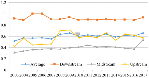
Figure 1. The IWRUE trends in the YREB and its downstream, midstream, and upstream
Figure 1 shows the IWRUE trends in the YREB and its upstream, midstream, and downstream. In the downstream, the IWRUE trend in the sample period could be divided into two different phases with 2008 as the dividing point: the IWRUE increased and then decreased before 2008, after that, the IWRUE remained stable, without any significant changes. In the midstream, the IWRUE increased slowly before 2016, but rose sharply from 2016 to 2017. In the upstream, the IWRUE fluctuated significantly before 2010, and remained stable afterwards.
Moreover, the three regions of the YREB also had a large gap in IWRUE. During the sample period, the IWRUE of the downstream averaged as high as 0.9168, far above the YREB average of 0.6009; the mean IWRUE of the midstream was only 0.3952, way below the YREB average; the mean IWRUE of the upstream was 0.5695, close to the YREB average. In short, the downstream achieved the highest IWRUE in the YREB, followed in turn by the upstream, and the midstream. This further confirms that the campaign for industrial water conservation must center on the upstream and midstream.
3.2 Estimation results of Tobit model
Based on the Tobit model (3), the effects of the influencing factors on YREB IWRUE were estimated on Stata 12. The regression results are recorded in Table 4.
Economic development (ED) has a positive impact on YREB IWRUE at the significance level of 1%, indicating that higher per-capita GDP promotes IWRUE. Without changing any other condition, every 1% growth of ED will increase the IWRUE by 0.2449%. On the one hand, economic development propels continued industrialization of the region, and promotes the modernization of industrial equipment, providing industrial enterprises with the material basis for water conservation. On the other hand, economic development motivates industrial enterprises to shift from extensive management to refined management, and reduce the intensity of water consumption, thereby lowering costs and enhancing competitiveness.
Table 4. The regression results of Tobit model
|
Variable |
Coefficient |
T-value |
P-value |
|
ED |
0.2449*** |
4.70 |
0.000 |
|
WE |
-0.3613*** |
-5.99 |
0.000 |
|
OS |
0.5022*** |
2.49 |
0.014 |
|
TP |
-4.7834** |
-1.94 |
0.054 |
|
OU |
0.8027*** |
7.13 |
0.000 |
|
GI |
-1.3148** |
-2.33 |
0.021 |
|
L- likelihood |
4.5392 |
||
Note: *, **, and *** are the significance levels of 10%, 5%, and 1%, respectively.
The estimated coefficient of water endowment (WE) was negative, passing the significance test at the 1% level, suggesting that more per-capita water resources suppresses YREB IWRUE. This reflects from the side that water-rich regions tend to have a low unit water price. Thus, industrial enterprises and other water users have a weak awareness of water conservation, and waste lots of precious water resources. The YREB is located in southern China, where water resources are relatively abundant. The unit water price in the region is relatively low. This obviously hinders the improvement of the IWRUE.
The ownership structure (OS) has a significant positive effect on YREB IWRUE. This means the IWRUE tends to increase with the industrial output of state-owned and state-controlled enterprises above the designated size as a proportion of the total industrial output. The possible reason is that, most state-owned and state-controlled enterprises in China are large enterprises. Unlike small and medium-sized private enterprises, these enterprises have advanced equipment, high production efficiency, and excellent water-saving and emission-reduction technologies. As a result, they can make intensive use of water resources.
Technological progress (TP) has a significant negative impact on YREB IWRUE on the level of 5%, that is, the growth in the internal R&D expenditure of industrial enterprises inhibits IWRUE improvement. The inhibitory effect is related to the resource allocation of R&D in industrial enterprises. Acemoglu et al. [21] divided the original technology R&D activities of industrial enterprises into clean technology-based activities and polluting technology-based activities, and noted the continuity between the two kinds of activities. In the real-world, many industrial enterprises prefer to invest more in polluting technology over clean technology, because the former requires relatively low investment and brings profits in the near future.
Opening-up (OU) exerted a significant promoting effect on YREB IWRUE, as its estimated coefficient was as high as 0.8027, passing the test on the 1% significance level. This falsifies the pollution haven hypothesis on industrial wastewater emissions. The import and export trade continues to develop in the YREB. The high foreign environmental standards for export products force industrial enterprises to reduce water consumption and pollution emissions by adopting intensive and green production processes. In this way, the industrial water environment can be effectively improved.
Government influence (GI) has a significant negative effect on YREB IWRUE. In other words, the IWRUE in the YREB decreased, when the local governments diverted more funds to agriculture, forestry, and water conservation.
This paper sets up a complete EIS for the IWRUE, and adopts the SBM with undesired output to measure the IWRUEs of the 11 YREB provinces in 2003-2017. In addition, the influencing factors of the IWRUE were analyzed by the Tobit model. The main conclusions are as follows:
First, the YREB provinces differed sharply in IWRUE through the sample period. Specifically, Shanghai and Zhejiang maintained their IWRUEs at the optimal level of 1; Jiangsu and Chongqing achieved satisfactory results on IWRUE, leaving a small room for improvement; Anhui, Sichuan, and Yunnan performed relatively good on IWRUE, but need further improvement; Jiangxi, Hubei, Hunan, and Guizhou had extremely poor performance in IWRUE, which must be greatly improved in future.
Second, the downstream, midstream, and upstream of the YREB witnessed different IWRUE trends in the sample period. Overall, the downstream provinces had higher IWRUEs than those in the upstream and midstream.
Third, the YREB IWRUE has a significant positive correlation with economic development, ownership structure, and opening-up, and a significant negative correlation with water endowment, technological progress, and government influence.
[1] Alnouri, S.Y., Linke, P., El-Halwagi, M. (2015). A synthesis approach for industrial city water reuse networks considering central and distributed treatment systems. Journal of Cleaner Production, 89: 231-250. https://doi.org/10.1016/j.jclepro.2014.11.005
[2] Filippini, M., Hrovatin, N., Zorić, J. (2008). Cost efficiency of Slovenian water distribution utilities: an application of stochastic frontier methods. Journal of Productivity Analysis, 29(2): 169-182. https://doi.org/10.1007/s11123-007-0069-z
[3] Wang, Y., Bian, Y., Xu, H. (2015). Water use efficiency and related pollutants' abatement costs of regional industrial systems in China: A slacks-based measure approach. Journal of Cleaner Production, 101: 301-310. https://doi.org/10.1016/j.jclepro.2015.03.092
[4] Pointon, C., Matthews, K. (2016). Dynamic efficiency in the English and Welsh water and sewerage industry. Omega, 58: 86-96. https://doi.org/10.1016/j.omega.2015.04.001
[5] Mortier, R., Block, C., Vandecasteele, C. (2007). Water management in the Flemish steel industry: the Arcelor Gent case. Clean Technologies and Environmental Policy, 9(4): 257-263. https://doi.org/10.1007/s10098-007-0102-y
[6] Krause, K., Chermak, J.M., Brookshire, D.S. (2003). The demand for water: Consumer response to scarcity. Journal of Regulatory Economics, 23(2): 167-191. https://doi.org/10.1023/A:1022207030378
[7] Deason, J.P., Schad, T.M., Sherk, G.W. (2001). Water policy in the United States: A perspective. Water Policy, 3(3): 175-192. https://doi.org/10.1016/S1366-7017(01)00011-3
[8] Nanere, M., Fraser, I., Quazi, A., D’Souza, C. (2007). Environmentally adjusted productivity measurement: An Australian case study. Journal of Environmental Management, 85(2): 350-362. https://doi.org/10.1016/j.jenvman.2006.10.004
[9] Hailu, A., Veeman, T.S. (2001). Non-parametric productivity analysis with undesirable outputs: an application to the Canadian pulp and paper industry. American Journal of Agricultural Economics, 83(3): 605-616. https://doi.org/10.1111/0002-9092.00181
[10] Seiford, L.M., Zhu, J. (2002). Modeling undesirable factors in efficiency evaluation. European Journal of Operational Research, 142(1): 16-20. https://doi.org/10.1016/S0377-2217(01)00293-4
[11] Tone, K. (2001). A slacks-based measure of efficiency in data envelopment analysis. European Journal of Operational Research, 130(3): 498-509. https://doi.org/10.1016/S0377-2217(99)00407-5
[12] Hu, J.L., Wang, S.C. (2006). Total-factor energy efficiency of regions in China. Energy Policy, 34(17): 3206-3217. https://doi.org/10.1016/j.enpol.2005.06.015
[13] Yao, X., Feng, W., Zhang, X., Wang, W., Zhang, C., You, S. (2018). Measurement and decomposition of industrial green total factor water efficiency in China. Journal of Cleaner Production, 198: 1144-1156. https://doi.org/10.1016/j.jclepro.2018.07.138
[14] Griliches, Z. (1986). Productivity R&D and basic research at firm level in the 1970’s. American Economic Review, 76(1): 141-153.
[15] Sahin, O., Stewart, R.A., Helfer, F. (2015). Bridging the water supply–demand gap in Australia: coupling water demand efficiency with rain-independent desalination supply. Water Resources Management, 29(2): 253-272. https://doi.org/10.1007/s11269-014-0794-9
[16] Wolfe, J.R., Goldstein, R.A., Maulbetsch, J.S., McGowin, C.R. (2009). An electric power industry perspective on water use efficiency. Journal of Contemporary Water Research & Education, 143(1): 30-34. https://doi.org/10.1111/j.1936-704X.2009.00062.x
[17] Romano, G., Guerrini, A. (2011). Measuring and comparing the efficiency of water utility companies: A data envelopment analysis approach. Utilities Policy, 19(3): 202-209. https://doi.org/10.1016/j.jup.2011.05.005
[18] Azad, M.A., Ancev, T., Hernández-Sancho, F. (2015). Efficient water use for sustainable irrigation industry. Water Resources Management, 29(5): 1683-1696. https://doi.org/10.1007/s11269-014-0904-8
[19] Cazcarro, I., Duarte, R., Sánchez-Chóliz, J. (2012). Water flows in the Spanish economy: Agri-food sectors, trade and households diets in an input-output framework. Environmental Science & Technology, 46(12): 6530-6538. https://doi.org/10.1021/es203772v
[20] Jin, W., Zhang, H.Q., Liu, S.S., Zhang, H.B. (2019). Technological innovation, environmental regulation, and green total factor efficiency of industrial water resources. Journal of Cleaner Production, 211: 61-69. https://doi.org/10.1016/j.jclepro.2018.11.172
[21] Acemoglu, D., Aghion, P., Bursztyn, L., Hemous, D. (2012). The environment and directed technical change. American Economic Review, 102(1): 131-166. https://doi.org/10.1257/aer.102.1.131