Jianchen Wang | Tao Jiang | Junquan Shen | Junhao Dai | Zequan Pan | Xiaolei Deng*
© 2020 IIETA. This article is published by IIETA and is licensed under the CC BY 4.0 license (http://creativecommons.org/licenses/by/4.0/).
OPEN ACCESS
This paper attempts to solve the insufficient machining precision of computer numerically controlled (CNC) machine tools, which is induced by the thermal error of the spindle. Firstly, the relationship between machining error and thermal sensitive points was analyzed through experiments. On this basis, the backpropagation neural network (BPNN) was improved by particle swarm optimization (PSO). Next, the improved network (PSO-BPNN) was used to build a thermal error compensation (TCE) model for the spindle of machine tools. Taking VM-500T precision machine tool as the object, the temperature data were grouped through the optimization based on thermal imaging, grey relational analysis (GRA), and fuzzy clustering, to determine the temperature sensitive items that causes the thermal error. To speed up network convergence, the PSO algorithm was introduced to optimize the number of hidden layers and the number of hidden layer nodes of the BPNN, lifting the network from the local optimum trap. To enhance the generalization ability, the weights and thresholds of the BPNN were also improved by the PSO. After that, two TCE models were established for the spindle of the machine tool, respectively based on the original BPNN and PSO-BPNN. Contrastive experiments show that the PSO-BPNN TCE model achieved the better generalization ability, and improved the prediction accuracy of the machining error of the CNC machine tool.
computer numerically controlled (CNC) machine tool, spindle, thermal error compensation (TEC), particle swarm optimization (PSO), backpropagation neural network (BPNN), prediction accuracy
Machine tool is the mother machine of all machineries. Its machining precision directly determines the precision of computer numerically controlled (CNC) machining products. The insufficient precision of CNC machine tool mainly comes from the thermal error induced by its changing temperature. In precision machining, 40-70% of all machining errors are attributable to the thermal error of machine tools [1-4]. The thermal error seriously restricts the manufacturing quality of machine tool.
Previous studies have proved that thermal error compensation (TEC) is a low-cost and efficient way to improve the machining precision of CNC machining tools, which does not need to change the original machine structure. Numerical method and modeling are two common approaches for TCE [4, 5]. Typical numerical methods include finite-element method and finite-difference method. Nevertheless, numerical methods are difficult to popularize, because the thermal error cannot be easily quantified under the constraints of thermal features and boundary conditions of the spindle.
Modeling aims to establish the thermal error model of the spindle, after the correlation between temperature and error at thermal sensitive points is obtained through numerous experiments and statistical analysis. In actual machining, however, the thermal drift of motorized spindle is highly variable, and the data samples on temperature and thermal drift are often small and imperfect, containing various fuzzy information [6-8]. Facing the small training samples, the common regression modeling methods, grey theory, and support vector machine (SVM) cannot fully comprehend the sample information, resulting in non-robust TEC models [9-13].
The artificial neural network (ANN) has been widely introduced to improve the robustness of the TEC models. For instance, Ramesh et al. [2] proposed a hybrid SVM-Bayesian network to classify the experimental data by working conditions, mapped the relationship between temperature and thermal error with SVM model, and accurately predicted the thermal error of spindle. Miao et al. [9] tested the temperatures and thermal errors at different spindle speeds, and learned that the multiple regression analysis (MRA) has poor prediction accuracy and robustness in the case of small modeling data. From the least squares SVM (LSSVM), Zhao et al. [10] derived the lifting wavelet transform-based LSSVM (LWT-LSSVM), making the thermal error model more stable and accurate in prediction. Ouafi et al. [11] optimized the backpropagation neural network with genetic algorithm (GA-BPNN), created a thermal error model based on five key temperature points, and demonstrated that the model could accurately forecast the thermal deformation at the turning center with a low computing load.
In addition, Ma et al. [12] grouped temperature variables through grey clustering and correlation analysis, and constructed a thermal error prediction model for high-speed spindle based on GA-BPNN. Drawing on grey theory and data preprocessing, Zhang et al. [13] presented a neural network (NN) TEC model for machine tools, and built a TEC model by repeatedly adjusting the data sequence length of the grey model as well as the weights and thresholds of the NN; the TEC model was found to have high prediction accuracy and strong robustness. After comparing human immune system with ANN, Yan et al. [14-17] proposed the artificial immune radial basis function (AIRBF) network, which boasts good adaptability and prediction accuracy through dynamic structural adjustment and online learning. Miao et al. [18] set up a state space modeling algorithm, and proved that the algorithm can automatically adjust the model as per the changing operating parameters of the machine tool, making the machine tool more adaptable.
The thermal drift of motorized spindle is complex, changeable, and nonlinear. The data on thermal drift and temperature, which are collected in the machining process, tend to be fuzzy and incomplete. Under various working conditions, the TEC of the spindle depends heavily on two factors: (1) The identification of thermal sensitive points, which bears on the accuracy of the TEC model; (2) The establishment of the TEC model, which reflects the exact relationship between the data collected from thermal sensitive points, and determines the accuracy and compensation ability of the TEC system.
This paper attempts to build a TEC model for VM-500T CNC machine tool. Firstly, the thermal sensitive points were selected through the optimization based on thermal imaging, grey relational analysis (GRA), and fuzzy clustering. Next, the BPNN was improved by particle swarm optimization (PSO), and improved network (PSO-BPNN) was used to build a TEC model for the spindle of the machine tool. Finally, the proposed model was proved feasible through the comparison with the original BPNN model in terms of accuracy and generalization ability.
2.1 PSO
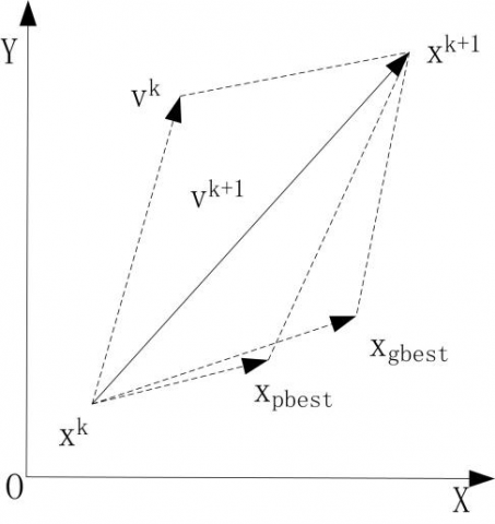
In the PSO algorithm [19], a number of particles are initialized randomly. Each particle is assigned a velocity and position. During the runtime, each particle keeps looking for the best-known individual velocity/position pbest in the search space, and updates its own velocity and position in comparison with the pbest values of others, thereby converging to the best-known global velocity/position gbest. The position/velocity of pbest and gbest is updated respectively by:
$\text{x}_{i,t+1}^{d}=x_{i,t}^{d}+x_{i,t+1}^{d}$ (1)
$\begin{align} & \text{v}_{i,t+1}^{d}=v_{i,t}^{d}+{{c}_{1}}*ran{{d}_{1}}*(p_{i,t}^{d}-x_{i,t}^{d}) \\ & +{{c}_{2}}*ran{{d}_{2}}*(p_{g,t}^{d}-x_{i,t}^{d}) \\ \end{align}$ (2)
where, $x_{i, t}^{d}$ and $v_{\mathrm{i}, \mathrm{t}}^{d}$ are the d-th dimension component of the position vector and the velocity vector of particle i in the t-th iteration, respectively; $p_{i, t}^{d}$ is the d-th dimension component of the pbest of particle i and the gbest of the swarm in the t-th iteration, respectively; $C_{1}$ and $C_{2}$ are the velocity update constants; rand $_{1}$ and rand $_{2}$, both fall in the interval of [0, 1] are random functions. The principle of particle movement is explained in Figure 1.
Figure 1. The principle of particle movement
The PSO algorithm is prone to fall into the local optimum trap, which dampens the optimization effect. To solve the problem, Shi et al. [20] introduced the inertia weight and constriction factor into the PSO algorithm. Subsequent studies have proved that introducing inertia weight brings equivalent benefits as introducing the constriction factor.
2.2 BPNN
The BPNN [20, 21] is known for its strong adaptability, self-learning ability, and relatively high prediction accuracy. However, the network might converge slowly in the later period, for the convergence relies on the gradient descent method. Besides, the network performance is greatly affected by the learning rate. If the learning rate is excessively high, the BPNN will oscillate significantly, rather than converge to the optimal solution. If the learning rate is too small, the BPNN will easily fall into the local optimum trap.
In general, the prediction ability of BPNN is positively correlated with its training ability. If the BPNN learns too many sample details, the overfitting phenomenon will occur. In this case, the training ability will be improved, but the prediction ability will be reduced. Then, the learned model could no longer reveal the statistical laws of the samples.
2.3 PSO-BPNN
To realize the fast convergence to the global optimal solution, the constriction factor was added to improve the convergence speed of the PSO; then, the number of hidden layers and number of hidden layer nodes were optimized to improve the prediction accuracy of the BPNN; finally, the PSO was combined with the BPNN to speed up the convergence of the network.
In the PSO-BPNN, the PSO performs global search, while the BPNN carries out the local search. The merits of the two techniques are combined to prevent the BPNN from falling into the local optimum trap. In addition, the weights and thresholds of the BPNN are corrected by the PSO, enhancing the generalization ability of the network [22, 23].
Based on the PSO-BPNN, the TCE model was created in the following steps:
Step 1. Data preprocessing
The temperature data and z-direction thermal deformation data were normalized to eliminate the singular values in the samples, which may otherwise prolong network training and slow down network convergence.
Step 2. Determining the structure and parameters of the BPNN
By formula (4), five combinations of temperature variables were selected (i.e. m=5). Only z-direction thermal deformation data and n-axis thermal deformation data were taken as 1.
Preliminary calculations indicate that the number of hidden layer nodes falls in the interval of [3, 13]. After comparing BPNNs with different number h of hidden layer nodes, the most suitable h value was found as 8. The default number of nodes of double hidden layers was also set to 8, and the number of output layer node was set to 1.
The BPNN parameters were configured as follows: the maximum number of training iterations is 300, the learning rate is 0.1, and the minimum training error is 0.0001.
Step 3. Determining PSO parameters.
After adding the constriction factor, the PSO algorithm can be updated as:
$v_{i,t+1}^{d}={{\chi }^{*}}\left( \begin{align} & v_{i,t}^{d}+c_{1}^{*}ran{{d}_{1}}^{*}\left( p_{i,t}^{d}-x_{i,t}^{d} \right) \\ & +{{c}_{2}}^{*}\text{ran}{{\text{d}}_{\text{2}}}^{*}\left( p_{g,t}^{d}-x_{i,t}^{d} \right) \\ \end{align} \right)$ (3)
where, χ is the constriction factor:
$\chi=\frac{2}{\left|2-\varphi-\sqrt{\varphi^{2}-4 \varphi}\right|}$ (4)
where, $\varphi=c_{1}+c_{2}$ and $\varphi>4$. Normally, the φ value is set to 4.1; c1 and c2 are set to 2.05. Substituting these values into formula (3), it was learned that $\chi=0.729$, and $c_{1}=c_{2}=0.729 * 2.05=1.49445$.
After the adjustment, the PSO parameters were configured as follows: the maximum number of iterations is 30, and the swarm size is 20. Then, the position and velocity of each particle were initialized.
Step 4. Weight and threshold adjustment and fitness calculation
The weights and thresholds of BPNN were adjusted by the PSO based on the constantly updated positions and velocities of particles. On this basis, the fitness was calculated to improve the particle position, particle velocity, as well as the weights and thresholds of the network. The fitness reflects the quality of each particle, and guides the subsequent updates of its position and velocity. The fitness function F can be expressed as:
$F=\sum\limits_{1}^{N}{\sum\limits_{1}^{L}{{{({{p}_{a,b}}-{{q}_{a,b}})}^{2}}}}$
where, N is the number of training samples; L was the number of output layer nodes; pa,b and qa,b are the expected output and actual output from the b-th node of the a-th sample, respectively.
The above formula shows that the smaller the fitness, the better the particle, and the smaller the network error.
Step 5. Iterative updates of position and velocity
Each particle iteratively updates its position and velocity based on its fitness, pbest and gbest by:
$\text{x}_{i,t+1}^{d}=x_{i,t}^{d}+x_{i,t+1}^{d}$ (5)
$\begin{align} & \text{v}_{i,t+1}^{d}=v_{i,t}^{d}+{{c}_{1}}^{*}\text{ran}{{\text{d}}_{\text{1}}}^{*}\left( p_{i,t}^{d}-x_{i,t}^{d} \right) \\ & +{{c}_{2}}^{*}\text{ran}{{\text{d}}_{\text{2}}}^{*}\left( p_{g,t}^{d}-x_{i,t}^{d} \right) \\ \end{align}$ (6)
where, $x_{i, t}^{d}$ and $v_{i, t}^{d}$ are the d-th dimension component of the position vector and the velocity vector of particle i in the t-th iteration, respectively; $p_{i, t}^{d}$ is the d-th dimension component of the pbest of particle i and the gbest of the swarm in the t-th iteration, respectively; $C_{1}$ and $C_{2}$ are the velocity update constants; rand $_{1}$ and rand $_{2}$, both fall in the interval of [0, 1] are random functions.
Step 6. Screening the particles meeting the output conditions
The particles whose fitness is below the set value or whose number of iterations is greater than the set value were outputted. Those failing to meet the output conditions would further update their positions and velocities until they meet these conditions.
Step 7. Optimizing the weights and thresholds for prediction
The optimal weights and thresholds were generated, and used to train the BPNN, laying the basis for the prediction of thermal error.
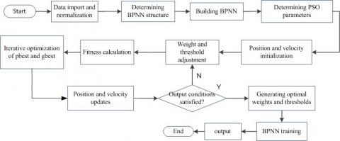
Through the above steps, the BPNN operation is effectively accelerated, and the prediction accuracy, convergence stability, and generalization ability of the network are improved. The workflow of PSO-BPNN is illustrated in Figure 2.
Figure 2. The workflow of PSO-BPNN
3.1 Selection of thermal sensitive points
As mentioned before, our experiments focus on the VM-500T CNC machine tool (maximum speed: 1,000r/min; horsepower of spindle motor: 3.7/5.5kW).
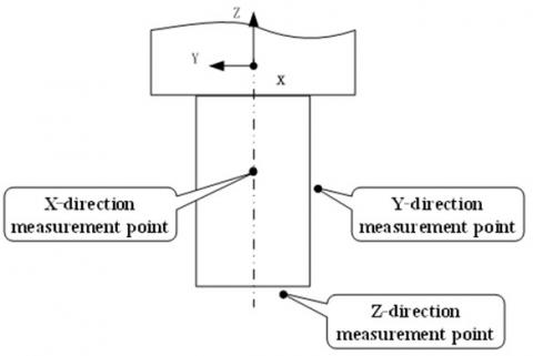
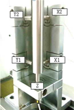
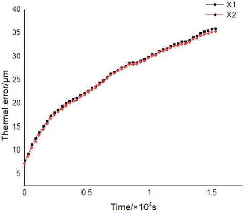
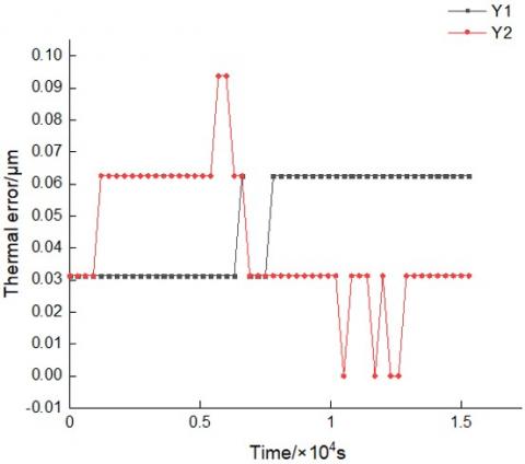
The thermal drift of spindle is usually determined by five-point measuring method [22, 23]. Hence, five points X1, X2, Y1, Y2, and Z (Figure 3) were selected to detect the spindle deformation. After multiple tests at different speeds and excluding the errors of initial positioning and radial alignment, it was found that the thermal offsets of the spindle in the x and y directions are very small, exerting a negligible impact on the machining precision.
Figures 4-6 provide the thermal deformations on the x-, y-, and z-directions, respectively. It can be seen that Z-direction deformation changed obviously with time, exerting a serious impact on the machining precision. Thus, the thermal error in the Z-direction was selected as the target of TCE modeling.
Figure 3. The arrangement of the five points
Figure 4. The thermal deformation in the x-direction
Figure 5. The thermal deformation in the y-direction
Figure 6. The thermal deformation in the z-direction
Figure 7. The thermal images
Then, thermal imaging [24] was adopted to detect the temperature change of the working spindle. Based on the detected results, several positions with obvious temperature rise were preliminarily selected as the key points, which reduces the experimental cost, eliminates the interference data, and improves the modeling accuracy.
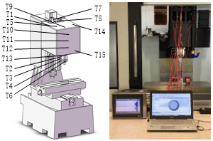
The thermal imaging was completed with a Fluke TiS50 infrared thermal imager (range: 10-50℃; distance: 1.5m; nominal temperature: 2%). The temperature was collected by two 8-channel temperature acquisition modules, which are embedded with a 16-bit analog/digital (A/D) conversion and photoelectric isolation device.
Multiple experiments were carried out with the machine tool in idle state. It was observed that the temperature rise around the spindle and the spindle housing is of experimental significance. The thermal images on the spindle and its end cap, sleeve and support are displayed in Figure 7 above.
Through the preliminary analysis on the thermal images, a total of 16 key points was selected for our experiments. Magnetic suction temperature sensors (resolution: 0.1℃; accuracy: 0.4℃; range: 0-100℃) were deployed on these points (Figure 8; Table 1).
Figure 8. The deployment of magnetic suction temperature sensors
Table 1. The positions of magnetic suction temperature sensors
|
Serial number |
Position |
|
T1, T5, T9, T14 |
Upper end of spindle box |
|
T10, T11, T12 |
Front end of spindle housing |
|
T15 |
Lower end of spindle box |
|
T2, T3, T4 |
Left side of spindle sleeve |
|
T13 |
Front end of spindle sleeve |
|
T6 |
Lower end of spindle sleeve |
|
T7, T8 |
Motor housing |
|
T16 |
Room temperature |
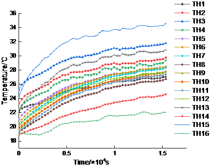
Figure 9. The temperature rise curves of the 16 sensors
The machine tool was kept idle at a certain speed. The temperature data were sampled at an interval of 1s. The sampled data with normal temperature rise in 16,000s were selected for analysis. Figure 9 presents the temperature rise on the 16 sensors. It can be seen that the temperatures at all sensors were continuously increasing; the increment and increasing rate are negatively correlated with the distance from the sensor to the spindle.
3.2 Optimization of thermal sensitive points
The data collected by so many sensors cannot be grouped accurately by fuzzy clustering. Thus, the measuring points were initially screened through GRA [20], which can reflect the degree of correlation between parent sequence and subsequences to a certain extent. Here, the temperature data were optimized with the thermal deformation induced by temperature rise as the parent sequence, and the 16 temperature datasets as subsequences. Firstly, the obtained data were normalized to the same interval:
${{g}_{q}}(e)=\frac{{{d}_{q}}(e)-\underset{e}{\mathop{min}}\,{{d}_{q}}(e)}{\underset{e}{\mathop{\max }}\,{{d}_{q}}(e)\underset{e}{\mathop{-min}}\,{{d}_{q}}(e)}$ (7)
(q=1,2,⋯,a; e=1,2,⋯,b)
where, g_{q}(e) is the normalized data; d_{q}(e) is the original data; $\underset{e}{\mathop min{{d}_{q}}}\,(e)$ and $\underset{e}{\mathop max{{d}_{q}}}\,(e)$are the minimum and maximum values of the original data, respectively.
Then, the correlation coefficient was calculated by
$\omega (\text{e})=\frac{{{\Delta }_{\min }}+\lambda {{\Delta }_{\max }}}{{{\Delta }_{o}}(e)+\lambda {{\Delta }_{\max }}}$ (8)
where, g_{0}(e) is the reference sequence; \lambda is the deviation coefficient (the value is usually 0.5); \Delta_{\min } \text { and } \Delta_{\max } are the minimum and maximum deviations, respectively; $\Delta_{0}(e)$ is the deviation of $d_{q}(e)$ from $g_{0}(e)$:
${{\Delta }_{o}}(e)={{d}_{q}}(e)-{{g}_{0}}(e)$ (9)
where, $d_{q}(e)$ is the deviation of the reference sequence.
The mean correlation coefficient was adopted to compute the degree of grey correlation:
$r({{g}_{0}},{{d}_{q}})=\frac{1}{n}\sum\limits_{k=1}^{n}{\omega }(e)$ (10)
Table 2 records the degree of grey correlations between the measuring points. The greater the numerical result, the closer the correlation between the subsequence and the parent sequence, and the stronger the correlation between temperature data and thermal error data. As shown in Table 2, the measuring points did not differ significantly in the degree of grey correlation. Based on the degree of grey correlation, the measuring points were sorted in descending order, and the first eight points were selected as the main measuring points: T3, T8, T9, T10, T11, T12, T13, and T15.
where, r(go, dq) is the correlation between subsequence go and parent sequence dq; n is the length of the reference sequence.
Table 2. The degree of grey correlations between the measuring points
|
Measuring point |
R |
Measuring point |
R |
|
T1 |
0.7567 |
T9 |
0.8116 |
|
T2 |
0.7847 |
T10 |
0.8146 |
|
T3 |
0.8108 |
T11 |
0.8149 |
|
T4 |
0.8049 |
T12 |
0.8174 |
|
T5 |
0.8063 |
T13 |
0.8391 |
|
T6 |
0.8089 |
T14 |
0.7910 |
|
T7 |
0.7969 |
T15 |
0.8225 |
|
T8 |
0.8538 |
T16 |
0.7739 |
Step 1. The temperature data $T=T_{1}, T_{2}, \cdots, T_{n}$ were preprocessed, and the temperature matrix was converted into an n×n distance matrix by the square form function in MATLAB.
Step 2. The distance between any two elements in the distance matrix was calculated by the pdist function in MATLAB.
Step 3. The calculated results were expressed as cluster trees by the linkage function, and classified into groups by the cluster function in MATLAB.
Step 4. The combinations of temperature variables were judged by the correlation coefficient and compound correlation coefficient. The correlation coefficient can be calculated by:
$R_{ij}^{2}=\frac{\sum\limits_{j=1}^{n}{({{T}_{ij}}-\overline{{{T}_{i}}})({{Z}_{j}}-\overline{{{Z}_{j}}})}}{{{\left[ {{\sum\limits_{j=1}^{n}{({{T}_{ij}}-\overline{{{T}_{i}}})}}^{2}}{{\sum\limits_{j=1}^{n}{({{Z}_{j}}-\overline{{{Z}_{j}}})}}^{2}} \right]}^{\frac{1}{2}}}}$ (11)
where, $T_{i j}$ is the j-th temperature variable at point i; $\overline{T_{i}}$ is the mean temperature at point i; Zj is the j-th displacement variable; $\bar{Z}_{J}$ is the mean displacement.
The compound correlation coefficient can be calculated by:
$R_{ij}^{2'}=1-\frac{n-1}{n-i-1}(1-R_{ij}^{2})$ (12)
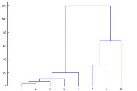
The fuzzy clustering process is explained in Figure 10 [26]; the calculation results of correlation coefficients and complex correlation coefficients are listed in Table 3.
Table 3. The correlations between main measuring points
|
Measuring point |
$R^{2}$ |
$R^{2^{\prime}}$ |
|
T3 |
0.8766 |
0.8764 |
|
T8 |
0.8284 |
0.8277 |
|
T9 |
0.8313 |
0.8303 |
|
T10 |
0.8581 |
0.8570 |
|
T11 |
0.8441 |
0.8426 |
|
T12 |
0.8692 |
0.8676 |
|
T13 |
0.9418 |
0.9410 |
|
T15 |
0.9851 |
0.9850 |
Figure 10. The grouping through fuzzy clustering
Note: Points 1-8 are T3, T8, T10, T11, T12, T13, and T15, respectively
3.3 Model error prediction
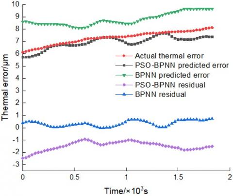
The temperature data collected at the five key measuring points were taken as inputs, and the z-direction thermal deformation as the output. The inputs were split into a training set of 14,000s, and a prediction set of 2,000s. The BPNN model and PSO-BPNN model were separately applied to predict the thermal errors. Figure 11 presents the running results of both models.
Figure 11. The thermal errors and residuals in the z- direction
As shown in Figure 11, the BPSO-BPNN model slightly outperformed the BPNN model, but the advantage is not obvious.
To verify the generalization ability of the PSO-BPNN, the input data were divided into a training set of 12,000s, a prediction set of 2,000s, and a verification set of 2,000s. The verification set was not used in BPNN construction or training, but used to simulate the network performance beyond the training. To ensure data consistency, the prediction part was excluded from image output. Then, the BPNN model and PSO-BPNN model were separately implemented, and their running results are displayed in Figure 12.
As shown in Figure 12, the PSO-BPNN significantly outshined the BPNN in generalization ability.
From Figures 11 and 12, the thermal error predicted by PSO-BPNN was closer to the actual value than that predicted by BPNN. Although both models achieved lower generalization ability than the prediction tasks, the PSO-BPNN was more accurate and stable than BPNN, and exhibited stronger prediction performance and generalization ability than the latter.
Figure 12. The generalization abilities in z-direction
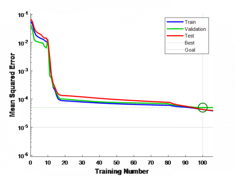
(a) Training error
(b) Regression results
Figure 13. The training performance of the BPNN
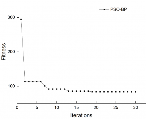
(a) Fitness function
(b) Training error
(c) Regression results
Figure 14. The training performance of the PSO-BPNN
Furthermore, the experiment data were automatically divided into a training set, a verification set, and a test set. BPNN and PSO-BPNN were separately trained on the training set, and verified on the verification set. The output error was obtained after the verification task. In addition, the data were automatically divided into the three sets again, and the results of BPNN and PSO-BPNN on these set were separately integrated into a comprehensive map. The training effect improves as the output approaches the Y-T diagonal. Figure 13 shows the training error and regression results of BPNN; Figure 14 shows the fitness, training error and regression result of PSO-BPNN.
From the fitness functions, it can be seen that BPNN and PSO-BPNN had the same target value, and their optimal value had the same gradient (10-5~10-4). Meanwhile, the training error of PSO-BPNN descended at a faster speed and for a shorter time than that of BPNN. The regression results show that the outputs of PSO-BPNN and BPNN were close to the said diagonal. The descent rates of fitness function reveal the superiority of PSO-BPNN in convergence speed and quality. Overall, PSO-BPNN can achieve a similar accuracy as BPNN, but at a faster convergence rate, in the same environment.
3.4 Results analysis
To display the optimization effect of PSO-BPNN more intuitive, the performance of the model was evaluated by mean relative error (MRE) and residual error. Let $a=(a(1), a(2), \cdots, a(n))$ be the residual data sequence, and $r=(r(1), r(2), \cdots, r(n))$ be the measured thermal errors. The MRE $\delta$ can be calculated by:
$\delta =\frac{\text{1}}{\text{n}}\sum\limits_{i=1}^{n}{\left| \frac{\text{a}(i)}{r(i)} \right|}$ (13)
where, $a(i)$ is the residual error of the model; $r(i)$ is the actual thermal error.
The residual error $\varepsilon$ can be calculated by:
$\varepsilon =\frac{\text{1}}{\text{n}}{{\sum\limits_{i=1}^{n}{(a(i)-\overline{a})}}^{2}}$ (14)
where, $\bar{a}$ is the mean residual error of the model.
The absolute difference between the predicted deformation and the actual deformation was divided by the absolute actual displacement to obtain the relative error. Then, the MRE was derived from the relative errors. Similarly, the relevant data were imported to formula (14) to obtain the residual error. The calculation results are shown in Table 4.
Table 4. The MRE and residual error of different models
|
Prediction method |
MRE$\delta / \%$ |
Residual errors $\mathcal{E}$ |
|
PSO-BPNN |
1.82% |
0.1702 |
|
BPNN |
6.74% |
0.4212 |
|
PSO generalization |
4.76% |
0.2347 |
|
BPNN generalization |
20.63% |
0.3652 |
This paper improves the BPNN with double hidden layers with the PSO, and applies the PSO-BPNN to compensate for the thermal error of the spindle of a CNC machine tool. The main conclusions are as follows:
(1) The GRA can screen the temperature data and identify the best combination of temperature variables, thereby reducing the experimental cost and improve the modeling accuracy.
(2) The PSO managed to improve the prediction accuracy, stability, and generalization ability of the BPNN.
(3) The PSO-BPNN could reduce the thermal error prediction error in the Z-direction of the spindle from 6.74% to 1.82% within the training range, and from 20.63% to 4.76% beyond the training range.
(4) The PSO-BPNN is a suitable algorithm for TEC modeling, and a desirable tool for TEC of the spindle of CNC machine tools.
This research was financially supported by Science and Technology Planning Project of Quzhou (No. 2020T024), Quzhou City - joint fund (No. LZY21E050002).
[1] Deng, X.L., Lin, H., Wang, J.C., Xie, C.X., Fu, J.Z. (2018). Review on thermal design of machine tool spindles. Optics and Precision Engineering, 26(6): 1415-1429. https://doi.org/10.3788/OPE.20182606.1415
[2] Ramesh, R., Mannan, M.A., Poo, A.N. (2000). Error compensation in machine tools—a review: Part I: geometric, cutting-force induced and fixture-dependent errors. International Journal of Machine Tools and Manufacture, 40(9): 1235-1256. https://doi.org/10.1016/S0890-6955(00)00009-2
[3] Ramesh, R., Mannan, M.A., Poo, A.N. (2002). Support vector machines model for classification of thermal error in machine tools. The International Journal of Advanced Manufacturing Technology, 20(2): 114-120. https://doi.org/10.1007/s001700200132
[4] Mayr, J., Jedrzejewski, J., Uhlmann, E., Donmez, M. A., Knapp, W., Härtig, F., Wendt, K., Moriwaki, T., Shore, P., Schmitt, R., Brecheer, C., Würz, T., Brecher, C. (2012). Thermal issues in machine tools. CIRP Annals, 61(2): 771-791. https://doi.org/10.1016/j.cirp.2012.05.008
[5] Ma, T.H., Jiang, L. (2018). Thermal error modeling of machine tools based on hybrid particle swarm optimization BP neural network. Chinese Journal of Construction Machinery, 16(3): 37-46.
[6] Singh, R.K., Sharma, R.V. (2018). Thermal performance of a co-axial borehole heat exchanger. Instrumentation Mesure Métrologie, 17(3): 443-453. https://doi.org/ 10.3166/I2M.17.455-466
[7] Morishima, T., van Ostayen, R., van Eijk, J., Schmidt, R. H.M. (2015). Thermal displacement error compensation in temperature domain. Precision Engineering, 42: 66-72. https://doi.org/10.1016/j.precisioneng.2015.03.012
[8] Blaise, K.K., Magloire, K.E.P., Prosper, G. (2018). Thermal performance evaluation of an indirect solar dryer. Instrumentation Mesure Métrologie, 17(1): 131-151. https://doi.org/10.3166/I2M.17.131-151
[9] Miao, E.M., Gong, Y.Y., Cheng, T.J., Chen, H.D. (2013). Application of support vector regression machine to thermal error modelling of machine tools. Optics and Precision Engineering, 21(4): 980-986. https://doi.org/10.3788/OPE.20132104.0980
[10] Zhao, J.L., Li, Q.L., Huang L.K. (2018). Research on thermal error modeling of CNC machine tools based on improved LSSV algorithm. Machinery Manufacturing and Automation, 47(6): 102-105. https://doi.org/10.19344/j.cnki.issn1671-5276.2018.06.024
[11] El Ouafi, A., Guillot, M. (2012). A comprehensive approach for thermal error model optimization for ANN-based real-time error compensation in CNC machine tools. In Applied Mechanics and Materials, 232: 639-647. https://doi.org/10.4028/www.scientific.net/AMM.232.639
[12] Ma, C., Zhao, L., Mei, X., Shi, H., Yang, J. (2017). Thermal error compensation of high-speed spindle system based on a modified BP neural network. The International Journal of Advanced Manufacturing Technology, 89(9-12): 3071-3085. https://doi.org/10.1007/s00170-016-9254-4
[13] Zhang, Y., Yang, J.G. (2011). Thermal error modeling of neural network machine tools based on gray theory pretreatment. Journal of Mechanical Engineering, 47(7): 134-139. https://doi.org/10.3901/JME.2011.07.134
[14] El Ouafi, A., Guillot, M., Barka, N. (2013). An integrated modeling approach for ANN-based real-time thermal error compensation on a CNC turning center. In Advanced Materials Research, 664: 907-915. https://doi.org/10.4028/www.scientific.net/AMR.664.907
[15] Yan, J.Y., Yang, J.G. (2009). Immune system based RBF neural network modeling for machine tool thermal error. Journal of Shanghai Jiaotong University, 1: 148-152.
[16] dos Santos, M.O., Batalha, G.F., Bordinassi, E.C., Miori, G.F. (2018). Numerical and experimental modeling of thermal errors in a five-axis CNC machining center. The International Journal of Advanced Manufacturing Technology, 96(5-8): 2619-2642. https://doi.org/10.1007/s00170-018-1595-8
[17] Hu, W.S., Sun, L. (2009). Model error compensation based on neural network method. Journal of Southeast University (English version), 25(3): 400-403. https://doi.org/10.3969/j.issn.1003-7985.2009.03.024
[18] Miao, E.M., Lu, X.X., Wei, X.Y., Song, X.J., Dong, Y.F. (2019). Thermal error modeling of CNC machine tools based on state space model. China Mechanical Engineering, 30(9): 45-51,60. https://doi.org/10.3969/j.issn.1004-132X.2019.09.006
[19] Kennedy, J., Eberhart, R. (1995). Particle swarm optimization. In Proceedings of ICNN'95-International Conference on Neural Networks, 4: 1942-1948. https://doi.org/10.1109/ICNN.1995.488968
[20] Shi, Y., Eberhart, R.C. (1999). Empirical study of particle swarm optimization. In Proceedings of the 1999 congress on evolutionary computation-CEC99 (Cat. No. 99TH8406), 3: 1945-1950. https://doi.org/10.1109/CEC.1999.785511
[21] Ma, T.H., Jiang, L. (2018). Thermal error modeling of machine tools based on hybrid particle swarm optimization BP neural network. Chinese Journal of Construction Machinery, 16(3): 221-224,230.
[22] Van Den Bergh, F., Engelbrecht, A.P. (2001). Training product unit networks using cooperative particle swarm optimisers. In IJCNN'01. International Joint Conference on Neural Networks. Proceedings (Cat. No. 01CH37222), 1: 26-131. https://doi.org/10.1109/IJCNN.2001.939004
[23] Ding, S., Su, C., Yu, J. (2011). An optimizing BP neural network algorithm based on genetic algorithm. Artificial Intelligence Review, 36(2): 153-162. https://doi.org/10.1007/s10462-011-9208-z
[24] ISO 230-3: 2007. (2007). Test code for machine tools–part 3: Determination of thermal effects, pp. 20-24.
[25] Wang, J.C., Lin, S.Q., Shen, Y.X., Xie, C.X., Deng, X.L. (2019). Research on thermal error measurement point optimization and modeling technology of CNC machine tool spindle. Aerospace Manufacturing Technology, 62(6): 41-46. https://doi.org/10.16080/j.issn1671-833x.2019.06.041
[26] Zhang, W., Ye, W.H. (2014). Optimization of temperature measuring points of machine tools based on grey correlation and fuzzy clustering. China Mechanical Engineering, 25(4): 456-460. https://doi.org/10.3969/j.issn.1004-132X.2014.04.006