Guiqing Xi | Caojun Huang* | Shiqi Liu
OPEN ACCESS
This paper designs a multi-sensor data fusion method for the nondestructive testing system using both ultrasonic sensors and magnetic flux leakage (MFL) sensors. Firstly, the detected data were fused by fuzzy linear regression and Dempster–Shafer theory (DST). Next, the fused results were presented intuitively by computing the fuzzy upper and lower bounds of the damage size in a certain interval of reliability and confidence. The application in several cases shows that our method can represent any test data in a form closer to the actual damage size, and display the fused data in an intuitive manner. The research findings have great applicable potential in many industries.
nondestructive testing, multi-sensor data fusion, Dempster–Shafer theory (DST), fuzzy linear regression
During nondestructive testing of oil pipelines, the quality of data collection and processing directly hinges on the sensor, the collection method and the data source [1]. In general, single-sensor data collection cannot obtain complete and precise data. The collected data are often highly uncertain, because each sensor has a unique level of quality, performance and noise [2, 3]. By contrast, multi-sensor data fusion reduces the data uncertainty through integration of data from multiple signals, making it easier to make robust decisions [4]. For example, multiple ultrasonic sensors and magnetic flux leakage (MFL) sensors can be coupled to make up for their respective defects and limitations, creating an effective nondestructive method to capture the abnormal parameters of oil pipelines [5, 6]. The combination between the two types of sensors can provide more accurate data for pipeline management and maintenance.
This paper designs a multi-sensor data fusion method capable of detecting wall thickness and pipe damage at any position, with a few number of ultrasonic sensors [7]. The fused data can approximate the actual size of damages, and thus improve the safety of oil pipelines [8, 9]. Example analysis shows that the proposed method did not mistake excessive damage for non-excessive damage, eliminating the need for costly and risky error checking.
The multi-sensor data fusion falls into three categories, namely, data level fusion, the feature level fusion, and the decision level fusion [10]. Among them, the feature level fusion can work flexibly and output precise results in real time, as it compresses the raw data and suppresses the interference. In this method, the fusion feature vectors of different test sources are integrated into a comprehensive feature vector [11]. The integration is achieved in two steps: extracting the amount or statistic is extracted from the data collected by each sensor, and analyzing the extracted information in a comprehensive manner [12]. Considering its advantages, the feature level fusion was adopted to design our multi-sensor data fusion algorithm.
The Dempster-Shafter theory (DST) was employed to fuse the data collected by ultrasonic sensors and the MFL sensors in our multi-sensor nondestructive testing system [13]. The application process is illustrated in Figure 1. In the DST, the basic probability assignment function, trust function and likelihood function of each evidence are computed, followed by the solving the three functions of the combination of all evidences; finally, the hypothesis of the maximum support under the joint action is selected according to certain decision-making rules.
In the nondestructive testing of oil pipeline, the author performed D-S evidence reasoning over the data collected by both ultrasonic and MFL sensors, and carried out the reasoning again on the fused data. The two-stage fusion process helps to rationalize the decision-making.
Considering the fuzziness of the data collected by multiple sensors, the fuzzy algorithm based on cognition model was introduced to process the multi-sensor fuzzy (MSF) data. Specifically, the uncertainty was expressed directly as fuzzy logic, and subjected to multivalve logic reasoning [14]. Next, the data fusion was realized by merging multiple propositions as per the fuzzy set theory of calculus.
Figure 1. Application of the DST in multi-sensor data fusion
(1) According to the DST, the confidence function of sensor i relative to the measure function of damage j can be expressed as:
$m_{i}(j)=\frac{C_{i}(j)}{\sum_{j} C_{i}(j)+N_{c}\left(1-R_{i}\right)\left(1-\omega \alpha_{i} \beta_{i}\right)}$ (1)
The measure function of the uncertainty θ of sensor i can be described as:
$m_{i}(\theta)=\frac{N_{c}\left(1-R_{i}\right)\left(1-\omega \alpha_{i} \beta_{i}\right)}{\sum_{j} C_{i}(j)+N_{c}\left(1-R_{i}\right)\left(1-\omega \alpha_{i} \beta_{i}\right)}$ (2)
where, ω is the performance coefficient of sensor i (e.g. geometry and surface roughness); αi is the maximum correlation coefficient between sensor i and each damage; βi is the distribution coefficient of sensor i; Ri is the reliability coefficient of sensor i; Nc is the type of damage.
Two confidence functions were cited to explain the fusion rule. In essence, the rule combines the probability assignments of two evidences under the same recognition framework into an overall probability assignment. Let mi(1) and mi(2) be the confidence functions relative to the measure functions of the two evidences under the same recognition framework, with the focal elements being A1, A2, ⋯, Ak and B1, B2, ⋯, Br, respectively. Then, we have:
$K=\sum_{i, j \atop A_{i} \cap B_{j}=\varphi} m_{1}\left(A_{i}\right) m_{2}\left(B_{j}\right)<1$ (3)
Then, the overall probability assignment can be expressed as:
$m(c)=\left[\begin{array}{l}{\Sigma_{i, j} \quad m_{1}\left(A_{i}\right) m_{2}\left(B_{j}\right)} \\ {\frac{A_{i} \cap B_{j}=c}{1-K}, \forall c \subset U} \\ {0, c=\varphi}\end{array}\right]$ (4)
(2) Damage membership, fuzzy interval and membership estimation. The values and probabilities of the same physical quantity measured by multiple sensors generally obey the normal distribution [15]. Hence, this paper takes the standard normal distribution function as the membership function of fuzzy set.
Through the analysis on the data collected by ultrasonic and MFL sensors, the estimated size z and the measured size z' of a damage has the following correlation:
$\phi(z)=\lambda_{0}+\lambda_{1} \phi\left(z^{\prime}\right)+\lambda_{2} \phi^{2}\left(z^{\prime}\right)+\cdots+\lambda_{m} \phi^{m}\left(z^{\prime}\right)+\varepsilon, \varepsilon \sim N\left(0, \sigma^{2}\right)$ (5)
where, the polynomial about ϕ(•)is the estimated size of the damage; ϕ(•)is the real function; ε is a normally-distributed error term; λi, i=1, 2, ⋯, m and σ2 are the parameters to be regressed.
In most cases, $\varphi(z)=\ln z, \varphi\left(z^{\prime}\right)=\ln z^{\prime}$ and $m=1$. Then, formula 5 can be converted into:
$\ln z=\lambda_{0}+\lambda_{1} \ln z^{\prime}+\varepsilon, \varepsilon \sim N\left(0, \sigma^{2}\right)$ (6)
The next step is to determine parameters λ0, λ1 and σ2. Let z1, z2, ⋯, zn and $Z_{1}^{\prime}, Z_{2}^{\prime}, \cdots Z_{n}^{\prime}$ be the estimated sizes and measured sizes of n damages, respectively. The n damages were assumed to subjected to an independent nondestructive test. It can be seen from regression analysis that the values of λ0 and λ1 can be estimated as:
$\hat{\lambda}_{0}=\frac{1}{n} \sum_{i=1}^{n} \ln z_{i}-\hat{\lambda}_{1} \frac{1}{n} \sum_{i=1}^{n} \ln z_{i}^{\prime}$ (7)
$\hat{\lambda}_{1}=\frac{\sum_{i=1}^{n}\left(\ln z_{i}-\frac{1}{n} \sum_{j=1}^{n} \ln z_{j}\right)\left(\ln z_{i}^{\prime}-\frac{1}{n} \sum_{j=1}^{n} \ln z_{j}^{\prime}\right)}{\sum_{i=1}^{n}\left(\ln z_{i}^{\prime}-\frac{1}{n} \sum_{j=1}^{n} \ln z_{j}^{\prime}\right)^{2}}$ (8)
The regression equation of the above formulas can be expressed as:
$\ln \tilde{z}=\hat{\lambda}_{0}+\hat{\lambda}_{1} \ln z^{\prime}$ (9)
where, $\tilde{Z}$ is the median size of the damage.
Then, the value of variance σ2 can be obtained by:
$\hat{\sigma}^{2}=\frac{1}{n-2} \sum_{i=1}^{n}\left(\ln z_{i}-\hat{\lambda}_{0}-\hat{\lambda}_{1} \frac{1}{n} \sum_{j=1}^{n} \ln z_{j}^{\prime}\right)^{2}$ (10)
Since the fuzzy membership function is assumed to obey standard normal distribution, the membership of the damage in the interval (0, z) can be derived from formulas (9) and (10) as:
$F(z | \hat{z})=\Phi\left[\left(\ln z-\hat{\lambda}_{0}-\hat{\lambda}_{1} \ln \hat{z}\right) / \hat{\sigma}\right]$ (11)
similarly, the membership of the damage in the interval [Z,+∞) can be expressed as:
$P(z | \hat{z})=1-F(z | \hat{z})$ (12)
where, Φ(•)is the standard normal distribution function; $F(z | \hat{z})$is the fuzzy distribution of the damage size in the detection range.
Substituting the measured size $\hat{z}$ of the said damage into formulas (9) and (10), the logarithm mean and the logarithm standard deviation can estimate as $\ln \tilde{z}=\hat{\lambda}_{0}+\hat{\lambda}_{1} \ln \hat{z}$. Hence, the lower and upper limits, $F_{L}\left(z_{0} | \hat{z}\right)=\Phi\left(u_{P L}\right)$ and $F_{U}\left(z_{0} | \hat{z}\right)=\Phi\left(u_{P U}\right)$, of the confidence γ of the damage relative to the membership interval (0,z0) can be obtained as:
$u_{P L}=\frac{\ln z_{0}-\ln \hat{z}}{\hat{\sigma}} \sqrt{\frac{2 v-2}{2 v-1}}-u_{\gamma} \sqrt{\frac{1}{n^{\prime}}+\frac{\left(\ln z_{0}-\ln \hat{z}\right)^{2}(2 v-2)}{\sigma^{2} \omega(2 v-1)}}$ (13)
$u_{P U}=\frac{\ln z_{0}-\ln \hat{z}}{\hat{\sigma}} \sqrt{\frac{2 v-2}{2 v-1}}+u_{\gamma} \sqrt{\frac{1}{n^{\prime}}+\frac{\left(\ln z_{0}-\ln \hat{z}\right)^{2}(2 v-2)}{\sigma^{2} \omega(2 v-1)}}$ (14)
$\omega=2\left|v+u_{\gamma}-c-\frac{1}{\sqrt{v+u_{\gamma}-c}}\right|$ (15)
similarly, the unilateral confidence of lower and upper limits of confidence γ relative to the membership interval [z0,+∞) can be derived as:
$P_{U}\left(z_{0} | \hat{z}\right)=1-\Phi\left(u_{P L}\right)$ (16)
$P_{L}\left(z_{0} | \hat{z}\right)=1-\Phi\left(u_{P U}\right)$ (17)
In nondestructive testing, the use of $F_{L}\left(z_{0} | \hat{z}\right)$ and $P_{U}\left(z_{0} | \hat{z}\right)$ can prevent the mistake of excessive damage for non-excessive damage, but cannot prevent the mistake of non-excessive damage for excessive damage. If the damage falls between the excessive level and the non-excessive level, more independent nondestructive tests should be conducted and the test results should be regressed repeatedly to increase the sample size n. Then, the confidence intervals $F_{U}\left(z_{0} | \hat{z}\right)-F_{L}\left(z_{0} | \hat{z}\right)$ and $P_{U}\left(z_{0} | \hat{z}\right)-P_{L}\left(z_{0} | \hat{z}\right)$ can be greatly shortened.
(3) Fuzzy data fusion of multiple data sources. Let $\hat{z}_{1}$ and $\hat{z}_{2}$ be the sizes of the same damage measured in two independent nondestructive tests. Substituting them into formula (11), the fuzzy distributions $F\left(z | \hat{z}_{1}\right)$ and $F\left(z | \hat{z}_{2}\right)$ of the damage size can be obtained as:
$F\left(z | \hat{z}_{1}\right)=\Phi\left[\left(\ln z-\hat{\lambda}_{0}-\hat{\lambda}_{1} \ln \hat{z}_{1}\right) / \hat{\sigma}\right]$ (18)
$F\left(z | \hat{z}_{2}\right)=\Phi\left[\left(\ln z-\hat{\lambda}_{0}-\hat{\lambda}_{1} \ln \hat{z}_{2}\right) / \hat{\sigma}\right]$ (19)
Then, the DST was applied to deduce the unilateral confidence lower limit of the membership in the interval (0, z0):
$F_{L}\left(z_{0} | \hat{z}_{1}, \hat{z}_{2}\right)=\frac{F_{L}\left(z_{0} | \hat{z}_{1}\right) F_{L}\left(z_{0} | \hat{z}_{2}\right)}{1-F_{L}\left(z_{0} | \hat{z}_{1}\right)-F_{L}\left(z_{0} | \hat{z}_{2}\right)+2 F_{L}\left(z_{0} | \hat{z}_{1}\right) F_{L}\left(z_{0} | \hat{z}_{2}\right)}$ (20)
similarly, $P_{U}\left(z_{0} | \hat{z}_{1}\right), P_{U}\left(z_{0} | \hat{z}_{2}\right)$, and the unilateral confidence limit of the membership interval [z0,+∞) can be derived by formula (14) as:
$P_{U}\left(z_{0} | \hat{z}_{1}, \hat{z}_{2}\right)=\frac{P_{U}\left(z_{0} | \hat{z}_{1}\right) P_{U}\left(z_{0} | \hat{z}_{2}\right)}{1-P_{U}\left(z_{0} | \hat{z}_{1}\right)-P_{U}\left(z_{0} | \hat{z}_{2}\right)+2 P_{U}\left(z_{0} | \hat{z}_{1}\right) P_{U}\left(z_{0} | \hat{z}_{2}\right)}$ (21)
Obviously, the number of independent testing sources is positively correlated with the number of iterations and the computing load.
3.2 Fuzzy representation of the size of the same damage measured by one type of sensors
Let $\hat{z}$ be the size of a damage on an oil pipeline measured by one type of sensors in a nondestructive test [16]. Then, the fuzzy distribution of the damage size can be expressed as: $F\left(z_{0}\right)=\Phi\left[\left(\ln z_{0}-\hat{\lambda}_{0}-\hat{\lambda}_{1} \ln \hat{z}\right) / \hat{\sigma}\right]$.
For the damage size, the upper limit and lower limit of reliability can be obtained respectively by:
$\ln z_{U}=\hat{\lambda}_{0}+\hat{\lambda}_{1} \ln \hat{z}+k_{R}\left(n^{\prime}, \nu\right) \hat{\sigma}$ (22)
$\ln z_{U}=\hat{\lambda}_{0}+\hat{\lambda}_{1} \ln \hat{z}-k_{R}\left(n^{\prime}, v\right) \hat{\sigma}$ (23)
where,
$k_{R}\left(n^{\prime}, v\right)=\frac{u_{R}+u_{\gamma} \sqrt{\frac{1}{n^{\prime}}\left(1-\frac{u_{\gamma}^{2}}{w}\right)+\frac{u_{R}^{2}}{w}}}{1-\frac{u_{\gamma}^{2}}{w}} \sqrt{\frac{2 v-1}{2 v-2}}$ (24)
$w=2\left(v+u_{\gamma}-0.64-\frac{1}{\sqrt{v+u_{\gamma}-0.64}}\right)$ (25)
where, ν=n-2.
3.3 Fuzzy representation of the sizes of the same damage measured by two type of sensors
In this paper, the MFL sensors and ultrasonic sensors are applied to measure the same damage interpedently. The measured data must satisfy the following formulas:
$\ln z=\sum_{i=1}^{2} r_{i} \lambda_{0 i}+\sum_{i=1}^{2} r_{i} \lambda_{1 i} \overline{(\ln \hat{z})}_{i}+\varepsilon$ (26)
$\varepsilon \sim N\left[0,\left(\frac{1}{\sigma_{1}^{2}}+\frac{1}{\sigma_{2}^{2}}\right)^{-1}\right]$ (27)
Compared with the measurement method in 3.2, the variance $\left(\frac{1}{\sigma_{1}^{2}}+\frac{1}{\sigma_{2}^{2}}\right)^{-1}$ of ln Z in this section is relatively small, indicating that different sensors can detect the same damage independently and accurately. The logarithm means of the measured sizes of ultrasonic sensors and the MFL sensors can be denoted as $\overline{(\ln \hat{z})_{1}}$ and $\overline{(\ln \hat{z})_{2}}$, respectively. If the sample space is sufficiently large, the actual statistics can be replaced by their respective statistical estimators:
$\hat{r}_{\mathrm{i}}=\frac{1 / \hat{\sigma}_{1}^{2}}{1 / \hat{\sigma}_{1}^{2}+1 / \hat{\sigma}_{2}^{2}}=\frac{\hat{\sigma}_{2}^{2}}{\hat{\sigma}_{1}^{2}+\hat{\sigma}_{2}^{2}}$ (28)
$\hat{r}_{2}=\frac{1 / \hat{\sigma}_{2}^{2}}{1 / \hat{\sigma}_{1}^{2}+1 / \hat{\sigma}_{2}^{2}}=\frac{\hat{\sigma}_{1}^{2}}{\hat{\sigma}_{1}^{2}+\hat{\sigma}_{2}^{2}}$ (29)
$\hat{\sigma}^{2}=\left(\frac{1}{\hat{\sigma}_{1}^{2}}+\frac{1}{\hat{\sigma}_{2}^{2}}\right)^{-1}$ (30)
$F(z | \hat{z})=\Phi\left[\frac{\ln z-\sum_{i=1}^{2} \hat{r}_{i} \hat{\lambda}_{0 i}-\sum_{i=1}^{2} \hat{r}_{i} \hat{\lambda}_{1 i} \overline{(\ln \hat{z})}_{i}}{\left(\frac{1}{\hat{\sigma}_{1}^{2}}+\frac{1}{\hat{\sigma}_{2}^{2}}\right)^{-\frac{1}{2}}}\right]$ (31)
Then, the upper and lower limits of the reliability can be expressed as:
$\ln z_{U}=\sum_{i=1}^{2} \hat{r}_{i} \hat{\lambda}_{0 i}+\sum_{i=1}^{2} \hat{r}_{i} \hat{\lambda}_{1 i} \overline{(\ln \hat{z})}_{i}+k_{R}\left(n^{\prime}, \nu\right)\left(\frac{1}{\hat{\sigma}_{1}^{2}}+\frac{1}{\hat{\sigma}_{2}^{2}}\right)^{-\frac{1}{2}}$ (32)
$\ln z_{L}=\sum_{i=1}^{2} \hat{r}_{i} \hat{\lambda}_{0 i}+\sum_{i=1}^{2} \hat{r}_{i} \hat{\lambda}_{1 i} \overline{(\ln \hat{z})}_{i}-k_{R}\left(n^{\prime}, v\right)\left(\frac{1}{\hat{\sigma}_{1}^{2}}+\frac{1}{\hat{\sigma}_{2}^{2}}\right)^{-\frac{1}{2}}$ (33)
where,
$k_{R}\left(n^{\prime}, v\right)=\frac{u_{R}+u_{\gamma} \sqrt{\frac{1}{n^{\prime}}\left(1-\frac{u_{\gamma}^{2}}{w}\right)+\frac{u_{R}^{2}}{w}}}{1-\frac{u_{\gamma}^{2}}{w}} \sqrt{\frac{2 v-1}{2 v-2}}$ (34)
$w=2\left(v+u_{\gamma}-0.64-\frac{1}{\sqrt{v+u_{\gamma}-0.64}}\right)$ (35)
where, ν=ν1+ν2, ν1=n1-2, ν2=n2-2.
4.1 Data fusion effect of fuzzy linear regression
The ultrasonic sensors were used to measure the damage size of a stainless-steel fitting of an oil pipeline. The measured results (Table 1) were compared with the actual damage sizes.
Table 1. Measured damage size by ultrasonic sensors (mm)
|
Serial number i |
1 |
2 |
3 |
4 |
5 |
6 |
7 |
8 |
9 |
10 |
11 |
12 |
|
True height of crack zi |
7.6 |
2.9 |
9.0 |
1.6 |
9.2 |
2.1 |
6.6 |
1.9 |
1.8 |
1.8 |
1.3 |
2.9 |
|
Crack detection heigh $Z_{i}^{\prime}$ |
9.0 |
1.5 |
10.0 |
1.0 |
8.0 |
1.5 |
6.0 |
1.5 |
1.5 |
2.0 |
1.0 |
1.0 |
The measured data were processed by the fuzzy linear regression algorithm. Then, the regression relationship between the measured and actual damage sizes can be expressed as:
$\ln \tilde{z}=0.4841+0.7434 \ln z$' (36)
The standard deviation can be estimated as: $\hat{\sigma}$=0.2728.
Let U be the space of q damages, denoted as $δ_i$, i=1,2,⋯q, in the oil pipeline. If the damage size of each damage was measured by ultrasonic sensors, then the membership of the measured damage sizes in [z0,+∞) can be obtained as:
$P_{i}\left(z_{0} | \hat{z}_{i}\right)=1-\Phi\left[\left(\ln z_{0}-0.4841-0.7434 \ln \hat{z}_{i}\right) / 0.2728\right]$
$i=1,2, \cdots q$ (37)
The measured damage size $\hat{z}_{i}$ thus obtained belongs to the membership interval of excessive damage size z0. If $P_{\min }\left(z_{0} | \hat{z}_{i}\right)=0.95$ is the street membership, then any damage with measured size $P_{i}\left(z_{0} | \hat{z}_{i}\right) \geq P_{\max }\left(z_{0} | \hat{z}_{i}\right)$ is an excessive damage.
Figure 2. Fused data curve vs. the curve of actual damage size
The test data in Table 1 were fused by formula (36). The fusion results in Figure 2 indicate that the fused data curve was close to the curve of actual damage size, which proves the effectiveness of our algorithm.
The fuzzy linear regression can also judge if a damage is of excessive size. Based on the above calculation, it is assumed that three independent ultrasonic tests were performed to detect the same damage in the same stainless-steel fitting. The damage sizes measured in the three tests were respectively $\hat{z}$=4.8mm, $\hat{z}$=4.2mm and $\hat{z}$=4.9mm. Under the confidence level of 95 %, the memberships of the damage sizes were respectively $P_{U}\left(z_{0}=5 | \hat{z}=4.8\right)$=77.34 %, $P_{U}\left(z_{0}=5 | \hat{z}=4.2\right)$=63.87 % and $P_{U}\left(z_{0}=5 | \hat{z}=4.9\right)$=79.10 %. Then, the three damage sizes were fused by formula (21) as z≥5mm, whose membership was $P_{U}\left(z_{0}=5 | \hat{z}=4.8,4.2,4.9\right)$=95.80 % under the confidence level of 95 %.
The comprehensive analysis shows that the damage size is greater than or equal to 5mm, that is, the size of excessive damage, at a certainty of 95.77 %. If the traditional method is adopted, then the variance or mean will indicate that the damage size is smaller than 5mm. However, the actual size of the damage on the stainless-steel fitting was 5.3mm. Hence, the proposed fuzzy linear regression data fusion method enjoys high accuracy and prevents the mistake of excessive damage for non-excessive damage.
4.2 Example analysis of fuzzy representation of damage size
The seam damage of a 16MnR steel fitting was measured by ultrasonic and the MFL sensors. The measured damage sizes (Table 2) and the actual size are compared below.
The measured data were processed by the proposed fuzzy linear regression algorithm. Then, the regression relationship between the measured and actual damage sizes can be expressed as:
$\ln \tilde{z}_{c h a o}=0.4456+0.8773 \ln z_{c h a o}^{\prime}$ (38)
The standard deviation of the damage size measured by ultrasonic sensors can be described as:
$\begin{aligned} \hat{\sigma}_{\text {chao}}=0.1593 & \\ & \ln \tilde{z}_{l o u}=0.2723+0.9278 \ln z_{l o u}^{\prime} \end{aligned}$ (39)
The standard deviation of the damage size measured by the MFL sensors can be described as: $\hat{\sigma}_{l o u}$=0.1835.
Based on the above formulas and the data in Table 2, the fused data curve is plotted and compared with the curve of actual damage size in Figure 3.
Table 2. Measured damage sizes by ultrasonic and the MFL sensors (mm)
|
Serial number |
Damage real size zi |
Ultrasonic testing data z1i |
Magnetic flux leakage test data z2i |
|
1 |
1.4 |
1.0 |
2.0 |
|
2 |
1.8 |
1.3 |
1.2 |
|
3 |
2.1 |
1.5 |
1.5 |
|
4 |
2.5 |
1.7 |
2.0 |
|
5 |
2.8 |
3.0 |
3.0 |
|
6 |
3.2 |
2.0 |
2.3 |
|
7 |
3.2 |
2.3 |
2.5 |
|
8 |
3.6 |
2.2 |
2.3 |
|
9 |
3.9 |
3.2 |
3.5 |
|
10 |
4.3 |
3.0 |
4.5 |
|
11 |
4.7 |
3.2 |
3.3 |
|
12 |
4.9 |
3.5 |
3.8 |
|
13 |
5.2 |
4.0 |
5.8 |
|
14 |
5.5 |
4.0 |
4.5 |
|
15 |
5.8 |
4.3 |
4.8 |
|
16 |
6.1 |
5.0 |
5.3 |
|
17 |
6.6 |
3.2 |
5.5 |
|
18 |
6.6 |
6.5 |
6.0 |
|
19 |
7.2 |
8.0 |
5.0 |
|
20 |
7.7 |
6.2 |
8.0 |
|
21 |
8.2 |
5.5 |
6.2 |
|
22 |
8.5 |
6.0 |
6.7 |
|
23 |
9.0 |
7.5 |
7.8 |
|
24 |
9.4 |
7.0 |
7.3 |
|
25 |
10.0 |
8.0 |
8.7 |
Figure 3. Fused data curve vs. the curve of actual damage size
Unlike the fused data curve of one type of sensors, the fused data curve of two types of sensors tracks the curve of actual damage size closely. This means the proposed data fusion method for the data collected by ultrasonic and the MFL sensors can reflect the actual situation well.
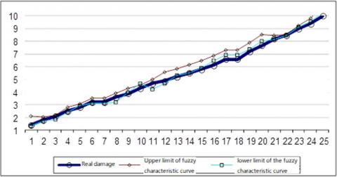
To evaluate the extent of damage, the fuzzy feature size of the data in Table was computed by formulas (32) and (33), and the results are displayed in Figure 4. Generally speaking, the lower bound of fuzzy feature size is closer to the actual size than the upper bound, but shows no specific correlation with the actual size. Hence, the upper bound is often adopted to judge the damage extent. According to the results in Figure 4, the lower bound curve of the fuzzy feature size coincided with the curve of actual damage size. This means the fuzzy feature size is consistent with the actual size.
Figure 4. Lower bound curve of fuzzy feature size vs. the curve of actual damage size
The data collected by ultrasonic and the MFL sensors exhibit heavy noises and high redundancy. To solve the problems, this paper designs a multi-stage data fusion method, which integrates fuzzy algorithm with linear regression, and relies on membership to describe damage size and judge if the damage is excessive. The application in several cases shows that our method can represent any test data in a form closer to the actual damage size, and display the fused data in an intuitive manner. Coupled with visual inspection and expert database, this algorithm can determine the exact size and type of damage, judge if the pipeline needs repairing or replacement, and disclose other important information. The research findings have great application potential in nondestructive testing for oil and gas transport and mining.
This research was funded by Science and Technology Program of Heilongjiang Province Agriculture and Reclamation Bureau of China (HNK125ABZD-05-18A, HNK125-06-02), and Science Fund Project of Heilongjiang Province (F201329, QC2014C078).
[1] Wang, W.H. (2013). Discussion on the development trend of ultrasonic nondestructive testing. Chemical Engineering and Equipment, 5: 164-166.
[2] Sorrente, B., Michau, V., Fleury, B., Conan, J.M., Sauvage, J.F. (2017). Measurement of the index field with a pyramidal sensor. Instrumentation Mesure Métrologie, 16(1-4): 213-228. https://doi.org/10.3166/i2m.16.1-4.213-228
[3] Ren, Z.H. (2016). Current situation and development trend of ultrasonic nondestructive testing technology. Technology and Market, 23(9): 255-256. http://dx.chinadoi.cn/10.3969/j.issn.1006-8554.2016.09.147
[4] Li, Y., Zheng, H., Jia, S.M., Liu, Q., Deng, K., Zhang, J. (2010). Development status of oil and gas pipeline inspection and monitoring technology at home and abroad. Petroleum Science and Technology Forum, 31(2): 30-35. http://dx.chinadoi.cn/10.3969/j.issn.1002-302x.2012.02.007
[5] Wang, B. (2018). Design of intelligent inspection robot for oil and gas pipeline defects based on ultrasonic wave. Modern Computer (Professional Edition), (28): 68-70. http://dx.chinadoi.cn/10.3969/j.issn.1007-1423.2018.28.017
[6] Wang, W.M., Wang, X.H., Zhang, S.M., Zeng, M., Wang, H.K. (2014). Long-distance pipeline ultrasonic internal inspection-state of the art. Oil & Gas Storage and Transportation, 33(1): 5-9. http://dx.chinadoi.cn/10.6047/j.issn.1000-8241.2014.01.002
[7] Yuan, X.P. (2013). Research and application of the velocity effect of the detector in the magnetic flux leakage pipeline, Shenyang. Shenyang University of Technology.
[8] Chen, W., Wang, B.L., Wang, B.T. (2018). Application and development of magnetic flux leakage testing technology in pipeline corrosion detection in China. Petrochemical Technology, 25(7): 223-330. http://dx.chinadoi.cn/10.3969/j.issn.1006-0235.2018.07.175
[9] Xu, L.L., Wang, J., Jiang, F.R. (2014). Theoretical study on velocity effect of detector in magnetic flux leakage pipeline. Science & Technology Vision, (4): 8-14. http://dx.chinadoi.cn/10.19694/j.cnki.issn2095-2457.2014.04.005
[10] Lin, W., Chu, S.N. (2015). Multi sensor data fusion technology for oil pipeline detection. Journal of Natural Science of Heilongjiang University, 32(3): 397-403. http://dx.chinadoi.cn/10.13482/j.issn1001-7011.2015.03.014
[11] Zhou, P. (2015). Research and prospect of multi-sensor data fusion technology. Internet of Things technology, 5(5): 23-25. http://dx.chinadoi.cn/10.16667/j.issn.2095-1302.2015.05.037
[12] Zhang, S.Q., Zhang, L., Duan, Y. (2003). A data fusion structure based on neural network and D-S inference and its application in ultrasonic testing. Journal of Sensor Technology, 16(1): 47-49. http://dx.chinadoi.cn/10.3969/j.issn.1004-1699.2003.01.012
[13] Liao, J.P. (2013). Multisensor data fusion based on D-S evidence theory and artificial neural networks. Journal of Convergence Information Technology, 8(8): 1070.
[14] Yang, D., Ji, H.B., Gao, Y.C. (2018). A robust D-S fusion algorithm for multi-target multi-sensor with higher reliability. Information Fusion, 47: 32-44. https://doi.org/10.1016/j.inffus.2018.06.009
[15] Černý, M., Hladik, M. (2018). Possibilistic linear regression with fuzzy data: Tolerance approach with prior information. Fuzzy Sets and Systems, 340: 124-144. http://dx.doi.org/10.1016/j.fss.2017.10.007
[16] Baskar, C., Nesakumar, N., Rayappan, J.B.B., Doraipandian, M. (2017). A framework for analysing E-Nose data based on fuzzy set multiple linear regression: Paddy quality assessment. Sensors and Actuators A: Physical, 267: 200-209. https://doi.org/10.1016/j.sna.2017.10.020