Wenjuan Huang | Wei Zhao* | Jin Zhang
OPEN ACCESS
This paper attempts to enhance the estimation accuracy of image Jacobian matrix, despite the impacts from unknown statistical features of process noise and measurement noise. For this purpose, the singular value decomposition aided Cubature Kalman filter (SVDCKF) was coupled with a noise compensator for visual servo systems based on the backpropagation neural network (BPNN). The proposed algorithm improves the accuracy of the Kalman filter and compensates for the two noise covariances through the nonlinear approximation function of the BPNN. The proposed Jacobian matrix estimation algorithm was subjected to a binocular stereo visual servoing experiment on the Motoman UP6 robot experimental platform. The experimental results show that the proposed algorithm is capable of completing servo positioning.
visual servo system, cubature Kalman filter, neural network, image Jacobian matrix
Thanks to the development of computer vision, the camera (visual sensor) has been widely adopted to serve as the “eyes” of robots [1]. The camera mainly captures images on the external environment. The information from the images was taken as the feedback signal to realize the closed-loop control of robot [2]. This process, known as visual servoing, has been applied in medical rescue and many other fields [3].
There are many ways to classify the visual servo systems in actual application [4, 5]. By system structure, the visual servo systems can be divided into eye-in-hand system and eye-to-hand system. By the number of cameras, the visual servo systems can be categorized as monocular, binocular and multi-eye systems. By feedback signal, the visual servo systems can be classified into position-based visual servoing (PBVS), image-based visual servoing (IBVS) and hybrid visual servoing.
Among them, the binocular stereo visual servo system with parallel optical axis stands out for its easy access to stereo information and excellent system performance. Meanwhile, the IBVS system is robust to camera calibration for the direct control of 2D images, eliminating the need to consider 3D reconstruction. As a result, the integration between the two types of systems has become increasingly popular in recent years [6].
The online estimation of image Jacobian matrix is fundamental to visual servo systems. Many scholars have applied Kalman filtering algorithm to estimate the matrix online using robot kinematics. For example, Reference [7] designs a Kalman filtering algorithm for online estimation of Jacobian matrix or homogenous transformation matrix of composite images, which can reduce the impact of noise. Reference [8] develops an adaptive Kalman filter to estimate the image Jacobian matrix of eye-in-hand servo system. Reference [9] constructs an improved Kalman filter for online estimation of Jacobian matrix. The Kalman filters in these studies boast strong applicability and recursiveness.
The Kalman filter can work perfectly in stochastic linear systems, provided that the model is accurate and that the system statistics and noises belong to Gaussian white noise sequences with known variance. However, visual servo systems will inevitably suffer from random noises, especially when the noise statistics are unknown. In this case, the traditional Kalman filter will perform poorly and even cause divergence [10].
To solve the problem, the Kalman filter can be fused with the neural network in two ways. One is to use the Kalman filter to improve the classification performance of the neural network. For instance, Reference [11] constructs a linear model based on the Kalman filter, and relies on it to improve the classification effect of the neural network through post-processing; the linear model ensures that the neural network predicts near-perfect output through linear combination of object features and the predicted output. This approach reduces the error and enhances the classification performance of the neural network.
The other is to better the filtering effect using the nonlinear approximation of the neural network. For example, Reference [12] adopts extended Kalman filter assisted artificial neural network to enhance the self-sensing capability of shape-memory alloy actuator. Specifically, the artificial neural network was employed to bridge the gap between the estimation by the extended Kalman filter and the actual stretch of the spring. Reference [13] investigates the data fusion of asynchronous, multi-rate and multi-sensor linear systems, and estimates the state vector using the neural network integrating multiple Kalman filters; The research results show that the integrated method outperformed the other ways of data fusion.
In our previous research [14], the singular value decomposition-aided cubature Kalman filter with neural network (NNSVDCKF) is compared with the singular value decomposition-aided cubature Kalman filter (SVDCKF) and standard Kalman filter (KF) in terms of the estimation of the image Jacobian matrix in an uncalibrated binocular stereo visual servo system for a 6DOF PUMA-560 robot. In this paper, the binocular stereo visual model and the NNSVDCKF are introduced in details, the image Jacobian matrix is estimated by the SVDCKF coupled with a backpropagation neural network (BPNN) noise compensator, and the proposed Jacobian matrix estimation algorithm is verified on the experimental platform for a Motoman UP6 robot.
2.1 Jacobian matrix
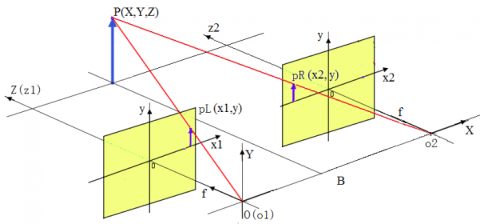
Figure 1. The binocular stereo visual model
As shown in Figure 1, the binocular stereo visual model is an eye-in-hand servo system. It is assumed that the two cameras have the same parameters, and their focal length f equals object distance; the origin O of the global coordinate system coincides with the optical center o1 of the left camera, which is parallel to the right one o2; the length between the two lens is denoted as B. In keeping with human habits, the imaging point is set at the front of the camera center. In addition, the left and right image planes are defined as x1-y1 and x2-y2, respectively. Since the two lenses are parallel to the installation, neither have a significant y-axis displacement. Hence, y1 can be considered as equal to y2, and both are denoted as y in this paper. According to the geometric relations in Figure 1, the change relationship between the position of feature points in the left and right image planes, and the position and pose of the end-effector [14]:
$\left[ \begin{matrix} {{{\dot{x}}}_{1}} \\ {\dot{y}} \\ {{{\dot{x}}}_{2}} \\\end{matrix} \right]=\left[ \begin{matrix} \frac{{{x}_{2}}-{{x}_{1}}}{B} & 0 & \frac{{{x}_{1}}({{x}_{1}}-{{x}_{2}})}{fB} & +\frac{{{x}_{1}}y}{f} & -\frac{{{f}^{2}}+{{x}_{1}}^{2}}{f} & +y \\ 0 & \frac{{{x}_{2}}-{{x}_{1}}}{B} & \frac{y({{x}_{1}}-{{x}_{2}})}{fB} & +\frac{{{f}^{2}}+{{y}^{2}}}{f} & -\frac{{{x}_{1}}y}{f} & -{{x}_{1}} \\ \frac{{{x}_{2}}-{{x}_{1}}}{B} & 0 & \frac{{{x}_{2}}({{x}_{1}}-{{x}_{2}})}{fB} & \frac{+y{{x}_{2}}}{f} & -\frac{{{f}^{2}}+{{x}_{1}}{{x}_{2}}}{f} & +y \\\end{matrix} \right]\cdot \left[ \begin{matrix} {{{\dot{S}}}_{X}} \\ {{{\dot{S}}}_{Y}} \\ {{{\dot{S}}}_{Z}} \\ {{{\dot{\theta }}}_{X}} \\ {{{\dot{\theta }}}_{Y}} \\ {{{\dot{\theta }}}_{Z}} \\\end{matrix} \right]$ (1)
where SX, SY and SZ are the position coordinates of the origin of the end-effector coordinate system; θX, θY and θZ are the space angles of the origin of the end-effector coordinate system.
let $p_{\text {single}}=\left[x_{1}, y, x_{2}\right]^{T}$ be the position matrix of the image feature points for a single object in the left and right image planes, and $U=\left[S_{X}, S_{Y}, S_{Z}, \theta_{X}, \theta_{Y}, \theta_{Z}\right]^{T}$ be the position and pose matrix of the end-effector in the global coordinate system. Then, Equation (1) can be extended to accommodate for multiple feature points:
$\dot{p}=\left[\begin{array}{c}{\dot{p}_{\text { single, } 1}} \\ {\dot{p}_{\text { single, } 2}} \\ {\dots} \\ {\dot{p}_{\text { single, } m}}\end{array}\right]= \left[\begin{array}{c}{J_{\text { single ,} 1}\left(p_{\text { single ,} 1}\right)} \\ {J_{\text { single ,} 2}\left(p_{\text { single ,} 2}\right)} \\ {\dots} \\ {J_{\text { single ,} m}\left(p_{\text { single ,} m}\right)}\end{array}\right] \dot{U} =J \dot{U}$ (2)
2.2. The estimation model for image Jacobian matrix
Based on the binocular stereo visual model in Section 2.1, the image Jacobian matrix should be solved before realizing the servoing of the mechanical arm. Here, the elements of the image Jacobian matrix are estimated by the positions of the image feature points. This calls for a process equation for the position of the state vector of the image Jacobian matrix and the measurement equation for the position of the image feature points.
Equation (2) can be discretized into:
$({{p}_{k+1}}-{{p}_{k}})/\Delta t=J\cdot \Delta {{U}_{k}}/\Delta t$ (3)
where $\Delta U_{k}$ is the changes of the position and pose matrix of the end-effector between moments k-1 and k. Then, the state vector $\chi_{k}$ and measurement vector $Z_{k}$ in each element of the image Jacobian matrix can be expressed as:
${{\chi }_{k}}=[{{J}_{1,1}},{{J}_{1,2}},...{{J}_{1,6}},{{J}_{2,1}},...{{J}_{m,6}}]_{18m\times 1}^{T}$ (4)
${{Z}_{k}}={{[{{p}_{k+1}}-{{p}_{k}}]}_{3m\times 1}}$ (5)
Then, the process equation and the measurement equation of the linear discrete dynamic system can be established as:
${{\chi }_{k+1}}={{\chi }_{k}}+\omega $ (6)
${{Z}_{k}}={{H}_{k}}\cdot {{\chi }_{k}}+\nu $ (7)
where $\omega_{18 m \times 1}$ is the process noise vector, an uncorrelated zero-mean Gaussian white noise sequence with covariance $Q_{18 m \times 18 m}$; $V_{3 m \times 1}$ is the measurement vector, whose covariance $R_{3 m \times 3 m}$ is defined the same as that of ω; $H_{k}$ is the measurement matrix:
$H_{k}=\left[\begin{array}{ccc}{\Delta \mathrm{U}_{\mathrm{k}}^{\prime}} & {\ldots} & {0} \\ {\ldots} & {\Delta \mathrm{U}_{\mathrm{k}}^{\prime}} & {\ldots} \\ {0} & {\ldots} & {\Delta \mathrm{U}_{\mathrm{k}}^{\prime}}\end{array}\right]$ (8)
3.1 SVDCKF
Consider a nonlinear discrete random state-space model in the following form:
${{x}_{k+1}}=f({{x}_{k}})+{{w}_{k}}$ (9)
${{Z}_{k+1}}=h({{x}_{k+1}})+{{v}_{k+1}}$ (10)
where $x_{k}$ is the n-dimensional system state vector; $Z_{k+1}$ is the m-dimensional measurement vector; $f(\cdot)$ is the state equation; $h(\cdot)$ is the measurement equation; $w_{k}$ is the zero-mean white noise with covariance matrices Q; $v_{k+1}$ is the zero-mean white noise with covariance matrices R. $w_{k}$ and $v_{k+1}$ are assumed to be uncorrelated with each other, and are not related to the initial state.
Then, the complete process of the SVDCKF algorithm can be explained as:
Step 1. Initialization
${{\hat{x}}_{0}}=E({{x}_{0}})$ and ${{\hat{P}}_{x,0}}=E(({{x}_{0}}-{{\hat{x}}_{0}}){{({{x}_{0}}-{{\hat{x}}_{0}})}^{T}})$ (11)
Step 2. Time update (k=0, 1, 2,…)
${{\hat{P}}_{x,k}}={{U}_{k}}\left[ \begin{align} & \begin{matrix} S_{k}^{*} & 0 \\\end{matrix} \\ & \begin{matrix} 0 & 0 \\\end{matrix} \\\end{align} \right]V_{k}^{T}$ (12)
${{\hat{X}}_{i,k}}={{U}_{k}}\sqrt{S_{k}^{*}}{{\xi }_{i}}+{{\hat{x}}_{k}}$ $i=1,2...2n$ (13)
${{\xi }_{i}}=\sqrt{n}{{[1]}_{i}}$ (14)
where [1]i is the i-th column of the point set [1].
${{\hat{X}}_{i,k+1/k}}=f({{X}_{i,k}})$ (15)
${{\hat{x}}_{k+1/k}}=\frac{1}{2n}\sum\limits_{i=1}^{2n}{{{{\hat{X}}}_{i,k+1/k}}}$ (16)
${{\hat{P}}_{x,k+1/k}}=(\frac{1}{2n}\sum\limits_{i=1}^{2n}{{{{\hat{X}}}_{i,k+1/k}}\hat{X}_{i,k+1/k}^{T}}-{{\hat{x}}_{k+1/k}}\hat{x}_{k+1/k}^{T})+Q$ (17)
Step 3. Measurement update
${{\hat{P}}_{x,k+1/k}}={{U}_{k}}\left[ \begin{align} & \begin{matrix} S_{k}^{*} & 0 \\\end{matrix} \\ & \begin{matrix} 0 & 0 \\\end{matrix} \\ \end{align} \right]V_{k}^{T}$ (18)
$X_{i,k+1/k}^{*}={{U}_{k}}\sqrt{S_{k}^{*}}{{\xi }_{i}}+{{\hat{x}}_{k+1/k}}$ $i=1,2...2n$ (19)
${{\hat{Y}}_{i,k+1/k}}=h(X_{i,k+1/k}^{*})$ (20)
${{\hat{Z}}_{k+1/k}}=\frac{1}{2n}\sum\limits_{i=1}^{2n}{{{{\hat{Y}}}_{i,k+1/k}}}$ (21)
${{\hat{P}}_{xZ,k+1/k}}=\frac{1}{2n}\sum\limits_{i=1}^{2n}{X_{i,k+1/k}^{*}{{({{{\hat{Y}}}_{i,k+1/k}})}^{T}}}-{{\hat{x}}_{k+1/k}}{{(\hat{Z}{}_{k+1/k})}^{T}}$ (22)
${{\hat{P}}_{Z,k+1/k}}=\frac{1}{2n}\sum\limits_{i=1}^{2n}{{{{\hat{Y}}}_{i,k+1/k}}{{({{{\hat{Y}}}_{i,k+1/k}})}^{T}}}-{{\hat{Z}}_{k+1/k}}{{({{\hat{Z}}_{k+1/k}})}^{T}}+R$ (23)
${{K}_{k+1}}={{\hat{P}}_{xZ,k+1/k}}{{\hat{P}}_{Z,k+1/k}}$ (24)
${{\hat{x}}_{k+1}}={{\hat{x}}_{k+1/k}}+{{K}_{k+1}}({{Z}_{k+1}}-{{\hat{Z}}_{k+1/k}})$ (25)
${{\hat{P}}_{x,k+1}}={{\hat{P}}_{x,k+1/k}}-{{K}_{k+1}}{{\hat{P}}_{Z,k+1/k}}K_{K+1}^{T}$ (26)
3.2 The BPNN noise compensator
A two-layer BPNN was selected as the noise compensator, and used to compensate for the covariance of system and measurement noises before each filtering process.
The inputs of the BPNN are the elements of the state estimation error $\Delta e_{\chi}$ and the innovation $V_{k}$ between the current moment k and moment (k-1):
$\Delta {{e}_{\chi }}={{\hat{\chi }}_{k}}-{{\hat{\chi }}_{k-1}}$ (27)
${{V}_{k}}={{Z}_{k}}-{{H}_{k}}{{\hat{\chi }}_{k-1}}$ (28)
The outputs of the BPNN are the compensated values p of Q and R at moment k, which are denoted as $\Delta Q_{k}$ and $\Delta R_{k}$, respectively. The two values can be obtained by training the BPNN with Sage-Husa method [15]. The values of f Q and R applied in Kalman filter at each moment can be calculated as:
${{Q}_{k}}(i,i)={{Q}_{k-1}}(i,i)+\Delta {{Q}_{k}}\begin{matrix} , & i=1,2,...,mn \\\end{matrix}$ (29)
${{R}_{k}}(i,i)={{R}_{k-1}}(i,i)+\Delta {{R}_{k}}\begin{matrix} , & i=1,2,...,n \\\end{matrix}$ (30)
where
$\Delta {{Q}_{k}}=\text{mean(}\sum\limits_{i=1}^{mn}{({{{\hat{Q}}}_{k-1}}(i,i)-{{Q}_{k-1}}(i,i)))}$ (31)
$\Delta {{R}_{k}}=\text{mean(}\sum\limits_{i=1}^{n}{({{{\hat{R}}}_{k-1}}(i,i)-{{R}_{k-1}}(i,i)))}$ (32)
3.3 The binocular stereo visual servo system with SVDCKF and BPNN noise compensator
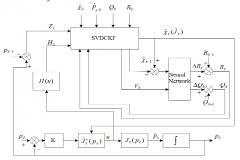
The binocular stereo visual servo system was modeled as shown in Figure 2. For simplicity, the following assumptions were put forward: (1) The internal and external parameters of the cameras are known. (2) The feature points of the object are always within the camera horizon. (3) The terminals of the robot arm coincide with the origin of the plane coordinate system of the left camera and the origin of the object coordinate system.
Figure 2. The structure of the proposed Jacobian matrix estimation algorithm
Theorem 1. Considering control plan in Figure 2 and kinematic servoing, the stable system control law under positioning control can be defined as:
$u=J{{(p)}^{+}}Ke=J{{(p)}^{+}}K({{p}_{d}}-p)$ (33)
where K is the positive definite matrix; $p_{d}$ is the current position; p is the desired position; e is the image error; $J(p)^{+}$ is the pseudo inverse of image Jacobian matrix.
Proof: The Lyapunov function can be defined as:
$V(t)=\frac{1}{2}({{e}^{T}}e)$ (34)
Taking the derivative of Equation (34), we have:
$\dot{V}(t)={{e}^{T}}\dot{e}$ (35)
The following can be derived from Equation (33):
$\dot{e}={{\dot{p}}_{d}}-\dot{p}=-\dot{p}=-J(p)u$ (36)
$\dot{V}(t)=-{{e}^{T}}J(p)u=-{{e}^{T}}J(p)J{{(p)}^{+}}Ke=-{{e}^{T}}Ke$ (37)
This means the proposed visual servo system is asymptotically stable in its workspace under the control law. In this case, the target image in the camera image plane coordinate system moves towards the desired position, and eventually stabilizes in the desired position. Thus, Theorem 1 is proved.
The proposed Jacobian matrix estimation algorithm was verified through a binocular stereo visual servoing experiment on the Motoman UP6 robot experimental platform.
The main hardware of the platform includes a Motoman UP6 arm, an XRC robot control cabinet, a control computer, two charge-coupled device (CCD) cameras and a DH-CG300 image acquisition card. The two cameras were mounted parallel to the end effector of the arm, forming the binocular vision model in Section 2.1, and moved along with the actuator.
The software of the platform was programmed under the VC++6.0 environment. The image acquisition module was implemented using the SDK in the DH-CG300 acquisition card. The feature matching module calls the function cvGoodFeaturesToTrack() provided by OpenCV. The image Jacobian matrix was estimated by the proposed SVDCKF with BPNN noise compensator. The generalized inverse matrix was calculated by the SVD function InversionSingularValue() in the class of matrix. The robot remote control module was accomplished by MotoCom32 library.
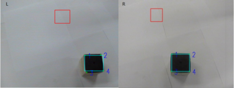
As shown in Figure 3, the experimental platform has a cube (side length: 5.4 cm) as the tracking object. The top surface of the cube was black and the other surfaces were in white, making it easy to match the feature points. The top four vertices of the cube were taken as feature points.
Figure 3. Experimental platform of binocular stereo visual servo system
The parameters of the two CCD cameras are as follows: lens size of 2.8 mm 1/3, general focal length of 303 pixels, the length between the two lens B=110 mm, the proportional gain K=1.25 and the image resolution of 400´300. The left camera was set as the origin of the arm coordinate system. In the robot coordinate system, the desired position at the end of the arm can be expressed as (1,012, 222, 609) (mm), and the initial angle as (158, -3, 28) (°). Meanwhile, the pixel coordinates of the feature points of the desired object are set as:
$\left[\begin{array}{l}{x_{1}} \\ {y_{1}} \\ {x_{2}} \\ {y_{2}}\end{array}\right]=\left[\begin{array}{cccc}{-16} & {34} & {-16} & {35} \\ {116} & {112} & {75} & {71} \\ {-89} & {-41} & {-99} & {-48} \\ {121} & {116} & {61} & {77}\end{array}\right]$
Figure 4. The desired and initial image positions of the object in binocular stereo visual servo system
Thus, we have:
${{p}_{d}}=\left[ \begin{matrix} {{x}_{1}} \\ y \\ {{x}_{2}} \\\end{matrix} \right]=\left[ \begin{matrix} -16 & 34 & -16 & 35 \\ 116 & 112 & 75 & 71 \\ -89 & 41 & -99 & -48 \\\end{matrix} \right]$
At the initial time, the position of the end of the arm in the robot coordinate system was (1,057, 76, 611) (mm); the initial angle was (158, 2, 30) (°).
Then, the pixel coordinates of the binocular image feature points are as follows:
$\left[\begin{array}{l}{x_{1}} \\ {y_{1}} \\ {x_{2}} \\ {y_{2}}\end{array}\right]=\left[\begin{array}{cccc}{85} & {139} & {92} & {114} \\ {39} & {-37} & {-97} & {-92} \\ {-16} & {45} & {-17} & {46} \\ {-34} & {-34} & {-93} & {-93}\end{array}\right]$
Thus, we have:
$p=\left[\begin{array}{c}{x_{1}} \\ {y} \\ {x_{2}}\end{array}\right]=\left[\begin{array}{cccc}{85} & {139} & {92} & {114} \\ {39} & {-37} & {-97} & {-92} \\ {-16} & {45} & {-17} & {46}\end{array}\right]$
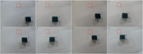
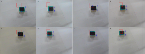
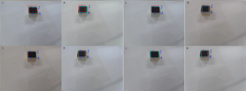
Figure 5. The image sequence captured by the binocular CCD cameras demonstrating the whole process of the visual servoing
The desired target image position (red square frame) and the initial image (green square frame) are shown in Figure 4. In the process of the visual servoing, the successive approximation images for the gradually approaching object are recorded in Figure 5. Obviously, the proposed algorithm can position the servo system.
Unlike monocular vision system, the binocular vision servo system eliminates the need for depth information. In practice, however, the estimation accuracy of image Jacobian matrix is affected by the unknown statistical features of process noise and measurement noise. In this paper, the SVDCKF is adopted to achieve a high filtering accuracy, and the BPNN is taken as a noise compensator to reduce the influence of the statistical features of uncertain noise to the filter. The proposed algorithm was proved as capable of completing servo positioning through an experiment on the Motoman UP6 robot experimental platform.
[1] Nelson, B.J., Papanikolopoulos, N.P., Khosla, P.K. (2015). Robotic visual servoing and robotic assembly tasks. IEEE Robotics & Automation Magazine, 3(2): 23-31. https://doi.org/10.1109/100.511777
[2] Mohebbi, A., Keshmiri, M., Xie, W. (2016). A Comparative study of eye-in-hand image-based visual servoing: Stereo vs. Mono. Journal of Integrated Design & Process Science, 19(3): 25-54. http://dx.doi.org/10.3233/jid-2015-0006
[3] Hom, B.K.P. (1996). Robot vision. Cambridge, Massachusetts: MIT Press.
[4] Pomares, J., Gil, P., Torres, F. (2010). Visual control of robots using range images. Sensors, 10(8): 7303-7322. https://doi.org/10.3390/s100807303
[5] Diosi, A., Segvic, S., Remazeilles, A., Chaumette, F. (2011). Experimental evaluation of autonomous driving based on visual memory and image-based visual servoing. IEEE Transactions on Intelligent Transportation Systems, 12(3): 870-883. https://doi.org/10.1109/TITS.2011.2122334
[6] Zhong, X.G., Zhong, X.Y., Peng, X.P. (2013). Robust Kalman filtering cooperated Elman neural network learning for vision-sensing-based robotic manipulation with global stability. Sensors, 13(10): 13464-13486. https://doi.org/10.3390/s131013464
[7] Wang, J.P., Liu, A., Tao, X.D., Chao, H. (2008). Microassembly of micropeg and -hole using uncalibrated visual servoing method. Precision Engineering, 32(3): 173-181.
[8] Xin, J., Bai, L., Liu, D. (2014). Adaptive Kalman filter-based robot 6DOF uncalibrated vision positioning. Journal of System Simulation, 26(3): 586-591.
[9] Wang, H.B., Li, P. (2009). On-line estimation for image Jacobin matrix based on improved Kalman filter. Journal of Wuhan University of Technology, 31(14): 145-148.
[10] Lv, X.D., Huang, X.H. (2006). Fuzzy adaptive Kalman filtering based estimation of image Jacobian for uncalibrated visual servoing. International Conference on Intelligent Robots and Systems, Beijing, China, pp. S2167-S2172. https://doi.org/10.1109/IROS.2006.282555
[11] Siswantoro, J., Prabuwono, A.S., Abdullah, A., Idrus, B. (2016). A linear model based on Kalman filter for improving neural network classification performance. Expert Systems with Applications an International Journal, 49(C): 112-122. https://doi.org/10.1016/j.eswa.2015.12.012
[12] Gurung, H., Banerjee, A. (2016). Self-sensing SMA actuator using extended Kalman filter and artificial neural network. Procedia Engineering, 144: 629-634. https://doi.org/10.1016/j.proeng.2016.05.054
[13] Safari, S., Shabani, F., Simon, D. (2014). Multirate multisensor data fusion for linear systems using Kalman filters and a neural network. Aerospace Science & Technology, 39: 465-471. https://doi.org/10.1016/j.ast.2014.06.005
[14] Zhao, W., Li, H.G., Zou, L.Y. (2016). Singular value decomposition aided cubature Kalman filter with neural network in uncalibrated binocular stereo visual servoing system. International Journal of Control and Automation, 9(12): 357-372.
[15] Shang, L., Liu, G.H., Zhang, R., Li, G.T. (2013). An adaptive Kalman filtering algorithm for autonomous orbit determination based-on BP neural network. Journal of Astronautics, 34(7): 926-931. http://dx.chinadoi.cn/10.3873/j.issn.1000-1328.2013.07.006