El Oualid Zouggar* | Souad Chaouch | Djaffar Ould Abdeslam | Abdelhamid Lilia Abdelhamid
OPEN ACCESS
The wind system based on double-fed induction generator (DFIG) has become a very important source of energy. To ensure the proper functioning of this system, many improved control algorithms have been developed for the rotor side converter (RSC). This article presents the analysis and design of a double-fed induction generator (DFIG) control technique based on coupling the type-2 fuzzy logic control with the sliding mode control (SMC). For the design of this technique, a decoupled modeling of the DFIG with the orientation of its stator flow is presented. The main purpose of the proposed technique is to make a control to meter the quantities of the powers produced by DFIG which are injected into the electrical network and to reduce the phenomenon of chattering which depends on control by sliding mode. This command has allowed us to reduce the chattering phenomenon and improve the performance of the system in terms of speed monitoring and stator side powers regulation. Simulations are performed using MATLAB / Simulink to validate the effectiveness of the proposed control algorithm. The simulation results, obtained when applying this control strategy to the system, demonstrated the validity of the results and thus validated the high performance of this control technique.
wind turbine- modeling - DFIG - powers regulation- sliding mode control- type-2 fuzzy logic control- robust control
The use of wind energy conversion systems has developed into one of the most important new alternatives to conventional fossil fuels in recent years. It offers an excellent opportunity to generate electricity and contribute to respect for the environment.
Recently, the use of doubly fed induction generator in global wind farms is very important because of its high performance in terms of systematic low cost, high energy efficiency, operating over a wide range of speed variation and extracting the maximum amount of power available [1-5]. In principle, the performance of the control system and the accuracy and response of the dynamic control system can be strongly influenced by factors such as changes in model variables, measurement errors, an online control system, load conditions and non-linearity.
However, the classical PID controller has been widely used to improve control system applications to consider these factors.
In order to solve the problem of parametric variations for the calculation of controllers in vector control, sliding mode control is highly appreciated in many areas among them the control of the wind system. It presents excellent properties, such as insensitivity to certain external disturbances and variation of parameters, sliding mode control (SMC) known for its simplicity and robustness [6].
Thanks to the inference system and expert knowledge, the design of the fuzzy logic controller can solve the problem of modeling and variations in system parameters.
Therefore the sliding mode control (SMC) has a disadvantage created by the discontinuous part of the control which is the effect of chattering.
The type 1 fuzzy logic controller gives better performance in DFIG control than traditional PI controllers [7-8]. In the general case the membership functions (MFs) and the bases of the rules are based on the experiences of experts or programmers. Therefore, there is uncertainty in the rules and the functions depend on the choices of the experts.
According to [9-12] fuzzy logic type 2 has advantages over fuzzy logic type 1 in handling uncertainties in memberships functions and in unexpected disturbances and is very much used in traffic [13], for power control [14], fault detection [15] and image processing [16] and control for Dual Star Induction Machine [17].
In order to eliminate the chattering phenomenon in the sliding mode control (SMC) and therefore improve its performance, this article includes the design of a controller based on the combination of the sliding mode controller with regulators based on the Type 2 fuzzy logic that replace the discontinuous part of the MSC.
This paper is organized as follows; modelling of the wind turbine as well as the Power Mechanical Regulation of a wind turbine are provided in section II. Sliding Mode control of the active and reactive powers is presented in section III. The fuzzy logic is introduced in section IV and the results simulation are presented and discussed in section V. Finally, a conclusion of the paper is presented in the last section.
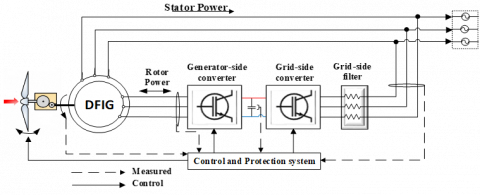
The wind energy conversion system is composed of the wind turbine, gearbox, DFIG and back-to-back converter. The Figure 1 shows the general structure of the wind energy conversion system with its studied control.
The turbine captures the wind's kinetic energy and transforms it into a torque that turns the rotor blades. Then, the DFIG converts the mechanical power into electrical power.
Figure 1. Synoptic diagram of the wind system
In this configuration, with the rotor-side converter control, it is possible to adjust the amplitude and frequency of the current in the rotor windings. So that the rotor speed can be changed over a wide range, thus allowing the system to: operate at a variable speed, recover maximum energy and improve its performance, and with the grid-side converter control, maintain the DC bus voltage at a desired reference value while keeping the reactive reference power at zero.
2.1 Wind turbine model
The power contained in the form of kinetic energy in the wind crossing at a speed Vv and surface A1, is expressed by: [18-19]
$P_{t}=\frac{1}{2} \rho A_{1} V_{v}^{3}$ (1)
where, ρ is the air density (kg/m3).
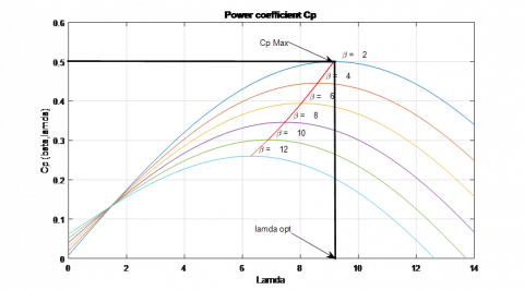
The wind turbine aerodynamics is characterized by the well-known non-dimensional curves of the power coefficient as a function of the peak speed ratio λ and the blade angle of inclination β [20].
The tip speed ratio is the ratio between the blade tip speed Ωt and the wind speed Vv can be expressed as follows [21]
$\lambda=\frac{\Omega_{t} R_{t}}{V_{v}}$ (2)
where, Ωt is the angular speed of the turbine rotor.
The expression of this power coefficient has been approached for this type of turbine, by the following equation [22-24]:
$C_{p}(\lambda, \beta)=(0.5-0.167(\beta-2))\sin \left[\frac{\pi(\lambda+0.1)}{18.5-0.3(\beta-2)}\right]-0.0018(\lambda-3)(\beta-2)$ (3)
The Figure 2 shows the relation between Cp, β and λ given by Eq. (3).
Figure 2. Curves of coefficients of power of a 4kW pitch regulated wind turbine, for different pitch angles $\beta$
From Figure 2, it can be seen that the power coefficient Cp is influenced by two parameters, both by the peak speed ratio $\lambda$ and by the pitch angle $\beta$. With Eq. (2). We can see that at a certain wind speed Vv, the power coefficient Cp can be set to be its maximum value by adjusting both the pitch angle $\beta$ and the rotation speed $\Omega_{t}$ of the turbine. As shown in Figure 2, when $\beta$ = 2 and $\lambda=\lambda_{\text { opt }}$, the power coefficient Cp will reach its maximum value Cp_max. The maximum theoretically achievable power coefficient is Cp_max=0.5.
Using the coefficient Cp, the wind turbine can recover only a part of that power: [24]
$P_{t}=\frac{1}{2} \rho \pi R_{t}^{2} V_{v}^{3} C_{p}(\lambda, \beta)$ (4)
where, Rt is the radius of the wind turbine and Cp represents the aerodynamic efficiency of the wind turbine.
The value of $\lambda$ corresponding to maximum of mechanical power available is called $\lambda_{\mathrm{opt}}$ (optimal). The rotor torque is obtained from the power received and the speed of rotation of the turbine:
$T_{t}=\frac{P_{t}}{\Omega_{t}}=\frac{\rho \pi R_{t}^{2} V_{v}^{3}}{2 \Omega_{t}} C_{p}(\lambda, \beta)$ (5)
The power transmission train is constituted by the blades linked to the hub, coupled to the slow shaft, which is linked to the gearbox, which multiplies the rotational speed of the fast shaft connected to the generator.
The turbine rotational speed and driving torque are expressed in the fast shaft by:
$\Omega_{m}=G \Omega_{t}$ (6)
$T_{m}=\frac{T_{t}}{G}$ (7)
where, G is the gearbox ratio.
The complete dynamic model of the wind system is compiled using the mechanical equation:
$J \frac{d \Omega_{m}}{d t}=T_{m}-T_{e m}-D \Omega_{m}$ (8)
where, J is the wind system inertia and D is the friction coefficient.
The block diagram of the wind turbine model is presented in Figure 3.
Figure 3. Wind turbine model
2.2 Mechanical regulation of the power of a wind system
The Eq. (4) makes it possible to establish a whole of characteristics giving the power available according to the number of revolutions of the generator for various speeds of wind.
Figure 4. Variations of the mechanical power available for a type of wind system given
Figures 4 and 5 plots the characteristics of the employed wind turbine model for simulations. It shows a generic power curve for a variable speed, and variable pitch wind turbine. At low wind speed (zone 2), the objective in this zone is to extract the maximum power with the application of a command that captures available wind energy. This command called MPPT. In zone III where the wind speed is increased, the power increases considerably, so we must apply a command that limits this power with the keep electricity production. This command based on the orientation of the blades of the wind turbine, it is called pitch control.
Figure 5. Law of optimal ordering of a wind system at variable speed
2.3 Maximum power tracking control strategy
In practice, a measurement of the wind speed is very difficult to achieve since the anemometer is located behind the rotor of the turbine and the diameter swept by the blades of the turbine is important.
In this operation region, the objective of the speed control is to follow the path of maximum power extraction.
When the turbine is working on the maximum power point,
$\lambda_{o p t}=\frac{R_{t} \Omega_{t}}{V_{v}}, C_{p}=C_{p_{-} \max }$
The aerodynamic torque extracted by the turbine is then given by [25]:
$T_{t}=\frac{\rho \pi R_{t}^{2}}{2 \Omega_{t}} \frac{R_{t}^{3} \Omega_{t}^{3}}{\lambda_{o p t}^{3}} C_{p_{-} \max }$ (9)
with:
$T_{t}=\frac{\rho \pi R_{t}^{5}}{2 \lambda_{o p t}^{3}} C_{p_{-} \max } \Omega_{t}^{3}=K_{o p t_{-} t} \Omega_{t}^{3}$ (10)
where:
$K_{o p t_{-} t}=\frac{\rho \pi R_{t}^{5}}{2 \lambda_{o p t}^{3}} C_{p_{-} \max }$
Thus as it is illustrated in the Figure (2), the maximum value of CP can be found using a graphical method, which is 0.5 in this case. This value corresponds to $\beta$ = 2 and $\lambda$ = 9.15. This tip speed value is assigned as the optimum tip speed. Based on this value, the optimum turbine speed curve at any given wind speed can be obtained. This curve is then used as a reference in the active power control.
The diagram block of the wind turbine model and its control are presented in Figure 6.
Figure 6. Wind turbine model with control
The doubly Fed Induction Generator is classically modeled in the Park d-q frame, giving rise to the equations system [24, 26]:
$\left\{\begin{array}{l}{V_{s d}=R_{s} I_{s d}+\frac{d \varphi_{s d}}{d t}-\omega_{s} \varphi_{s q} } \\ {V_{s q}=R_{s} I_{s q}+\frac{d \varphi_{s q}}{d t}+\omega_{s} \varphi_{s d} } \\ {V_{r d}=R_{r} I_{r d}+\frac{d \varphi_{r d}}{d t}-\omega_{r} \varphi_{r q} } \\ {V_{r q}=R_{r} I_{r q}+\frac{d \varphi_{r q}}{d t}+\omega_{r} \varphi_{r d} } \\ {\varphi_{s d}=L_{s} I_{s d}+L_{m} I_{r d} } \\ {\varphi_{s q}=L_{s} I_{s q}+L_{m} I_{r q} } \\ {\varphi_{r d}=L_{r} I_{r d}+L_{m} I_{s d} } \\ {\varphi_{r q}=L_{r} I_{r q}+L_{m} I_{s q} } \\ {T_{e m}=p \frac{L_{m}}{L_{s}}\left(I_{r d} \varphi_{s q}-I_{r q} \varphi_{s q}\right) }\end{array}\right.$ (11)
The active and reactive stator powers are given as follows:
$\left\{\begin{array}{l}{P_{s}=V_{s d} I_{s d}+V_{s q} I_{s q}} \\ {Q_{s}=V_{s q} I_{s d}-V_{s d} I_{s q}}\end{array}\right.$ (12)
The rotor currents that provide independent control of the active power Psand the reactive power Qs of the DFIG must be defined in the stator flux-oriented reference frame. Then the reference rotor currents are determined by the reference active and reactive power values.
For obvious reasons of simplification, the DFIG control is carried out in a frame dq related to the rotating field of the stator, in which the axis d is aligned, in this case, with the stator flux space vector, as shown in Figure (7), and a stator flux aligned with the axis d has been adopted. In addition, the stator resistance can be neglected because this is a realistic assumption for generators used in wind power [6, 27].
Figure 7. Synchronous rotating dq reference frame aligned with the stator flux space vector
On the basis of these considerations, we obtain the system of equations:
The objective is to apply this control to control independently of the active and reactive powers generated by the doubly fed induction generator by orientation from fluxes.
The reactive power set point will be kept zero so as to keep a unit power factor on the stator side.
$\left\{\begin{array}{l}{V_{s d}=0} \\ {V_{s q}=\omega_{s} \varphi_{s d}} \\ {V_{r d}=R_{r} I_{r d}+\frac{d \varphi_{r d}}{d t}-\omega_{r} \varphi_{r q}} \\ {V_{r q}=R_{r} I_{r q}+\frac{d \varphi_{r q}}{d t}-\omega_{r} \varphi_{r d}} \\ {T_{e m}=-p \frac{L_{m}}{L_{s}} I_{r q} \varphi_{s d}}\end{array}\right.$ (13)
Adaptation of Eq. (12) to our simplifying assumptions gives:
$\left\{\begin{array}{l}{P_{s}=-V_{s} \frac{L_{m}}{L} I_{r q}} \\ {Q_{s}=\frac{V_{s} \varphi_{s}}{L_{s}}-\frac{V_{s} L_{m}}{L_{s}} I_{r d}}\end{array}\right.$ (14)
The reactive power desired is
$Q_{s_{-} r e f}=0$ (15)
Using Eq. (14) and Eq. (15), we get the instruction
$\left\{\begin{array}{l}{I_{r q_{-} r e f}=-\frac{L_{s}}{V_{s} L_{m}} P_{s_{-} r e f}} \\ {I_{r d_{-} r e f}=\frac{V_{s}}{\omega_{s} L_{m}}}\end{array}\right.$ (16)
From Eq. (11), the relationship between the rotor currents and the voltages is obtained:
$\left\{\begin{array}{l}{\frac{d I_{r d}}{d t}=\frac{1}{L_{r} \sigma}\left(V_{r d}-R_{r} I_{r d}-\frac{L_{m}}{L_{s}} \frac{d \varphi_{s}}{d t}+\omega_{r} L_{r} \sigma I_{r q}\right)} \\ {\frac{d I_{r q}}{d t}=\frac{1}{L_{r} \sigma}\left(V_{r q}-R_{r} I_{r q}-\omega_{r} L_{r} \sigma I_{r d}-\omega_{r} \frac{L_{m}}{L_{s}} \varphi_{s}\right)}\end{array}\right.$ (17)
The lateral grid-side converter (CSR) and the filter illustrated in Figure 1 can be modeled in the Park d-q frame by the following equations:
$\left\{\begin{array}{l}{V_{f d}=R_{f} I_{f d}-L_{f} \frac{d I_{f d}}{d t}+\omega_{s} L_{f} I_{f q}+V_{g d}} \\ {V_{f q}=R_{f} I_{f q}-L_{f} \frac{d I_{f q}}{d t}+\omega_{s} L_{f} I_{f d}+V_{g q}}\end{array}\right.$ (18)
where,
represent the grid voltage, represent the grid current, represents the filter inductance and represents the filter resistance.The voltage across the DC bus capacitor is obtained by integrating the current flowing through the capacitor
$\frac{d V_{c}}{d t}=\frac{1}{c} I_{c}$ (19)
The active and reactive powers generated by the CSR are defined by:
$\left\{\begin{array}{l}{P_{f}=V_{f d} I_{f d}+V_{f q} I_{f q}} \\ {Q_{f}=V_{f q} I_{f d}-V_{f d} I_{f q}}\end{array}\right.$ (20)
4.1 Sliding mode control
The design of the sliding mode control is realized mainly in three complementary stages defined by [29-30]:
(1) Choice of sliding surfaces
Slotine proposes [26] a surface of sliding which is a scalar function such that the controlled variable slips on the surface:
$s(x)=\left(\frac{d}{d t}+\lambda\right)^{r-1} e(x)$ (21)
where, r is the relative degree of the system, λ is a positive constant and e(x) is the error between the variable and its reference. We will take r=1 for the command of the power we get:
$s(x)=e(x)$ (22)
The active power will be directly proportional to the axis q rotor current and reactive power proportional to the rotor axis current d.
$\left\{\begin{array}{l}{s(P)=e(p)=I_{r q_{-} r e f}-I_{r q}} \\ {s(Q)=e(Q)=I_{r d_{-} r e f}-I_{r d}}\end{array}\right.$ (23)
Then we will have:
$\left\{\begin{array}{l} {\dot{s}(p)=-\frac{L_{s}}{V_{s} L_{m}} \dot{P}_{s_{-} r e f}-\frac{1}{L_{r} \sigma}\left(V_{r q}-R_{r} I_{r q}-\omega_{r} L_{r} \sigma I_{r d}\right.-\omega_{r} \frac{L_{m}}{L_{s} \varphi_{s}}} \\ {\dot{s}(Q)=-\frac{V_{s}}{\omega_{s} L_{m}}-\frac{1}{L_{r} \sigma}\left(V_{r d}-R_{r} I_{r d}-\frac{L_{m}}{L} \frac{d \varphi_{s}}{d t}\right.+\omega_{r} L_{r} \sigma I_{r q}}\end{array}\right.$ (24)
(2) Conditions for convergence
In order to force the chosen variables to converge to their reference values it needs that both surfaces of sliding are driven to zero.
$\left\{\begin{array}{l}{s(p)=0} \\ {s(Q)=0}\end{array} \Rightarrow\left\{\begin{array}{l}{\dot{s}(P)=\frac{d}{d t}\left(I_{r q_{-} r e f}-I_{r q}\right)=0} \\ {\dot{s}(Q)=\frac{d}{d t}\left(I_{r d_{-} r e f}-I_{r d}\right)=0}\end{array}\right.\right.$ (25)
Control law design
Now consider the following command:
$\left\{\begin{array}{l}{\dot{s}(P)=-\operatorname{sgn}(s(P))} \\ {\dot{s}(Q)=-\operatorname{sgn}(s(Q))}\end{array}\right.$ (26)
Combining Eq. (26) with Eq. (24), we obtain
$\left\{\begin{array}{l}{\frac{L_{s}}{v_{s} L_{m}} \dot{P}_{s_{-} r e f}+\frac{1}{L_{r} \sigma}\left(V_{r q}-R_{r} I_{r q}-\omega_{r} L_{r} \sigma I_{r d}-\omega_{r} \frac{L_{m}}{L_{s}} \varphi_{s}\right)=\operatorname{sgn}(s(p)) } \\ {\frac{1}{L_{r} \sigma}\left(V_{r d}-R_{r} I_{r d}-\frac{L_{m}}{L_{s}} \frac{d \varphi_{s}}{d t}+\omega_{r} L_{r} \sigma I_{r q}\right)=\operatorname{sgn}(s(Q)) } \end{array}\right.$ (27)
Using the above equations, the rotor voltages are obtained
$\left\{\begin{array}{l}{V_{r q}=R_{r} I_{r q}+\omega_{r} L_{r} \sigma I_{r d}+g \frac{L_{m} V_{s}}{L_{s}}+\sigma L_{r} \dot{I}_{r e_{-} r e f}+L_{r} \sigma \operatorname{sgn}(s(P)) } \\ {V_{r d}=R_{r} I_{r d}-\omega_{s} g L_{r} \sigma I_{r q}+L_{r} \sigma \operatorname{sgn}(s(Q)) } \end{array}\right.$ (28)
The algorithm of control is defined by the relation:
$\left\{\begin{array}{l}{V_{r q}=V_{r q_{-} E q}+V_{r q_{-} a t t r}} \\ {V_{r d}=V_{r d_{-} E q}+V_{r d_{-} a t t r}}\end{array}\right.$ (29)
with
$\left\{\begin{array}{l}{V_{r q_{-} a t t r}=-v_{1} \operatorname{sat}(s(P))} \\ {V_{r d_{-} a t t r}=-v_{2} \operatorname{sat}(s(Q))}\end{array}\right.$ (30)
Therefore, combining these equations with Eq. (28), we obtain
$\left\{\begin{array}{l}{V_{r q_{-} a t t r}=L_{r} \sigma \operatorname{sgn}(e(P))} \\ {V_{r d_{-} a t t r}=L_{r} \sigma \operatorname{sgn}(e(Q))}\end{array}\right.$ (31)
$\left\{\begin{array}{l}{V_{r q, E q}=R_{r} I_{r q}+\omega_{r} L_{r} \sigma I_{r d}+g \frac{L_{m} V_{s}}{L_{s}}+\sigma L_{r} \dot{I}_{r q_ {-} r e f}} \\ {V_{r d, E q}=R_{r} I_{r d}-\omega_{s} g L_{r} \sigma I_{r q}}\end{array}\right.$ (32)
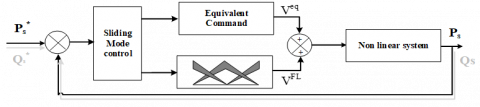
Finally, the global sliding control system is grouped in the Figure 8.
Figure 8. Schematic diagram of the sliding mode control system
4.2 Fuzzy logic control
Since Zadeh [31] first introduced fuzzy set theory, Fuzzy logic control (FLC) has been successfully applied in various fields.
Basically, the use of fuzzy logic control for a system is based on rules that are based on the expertise and knowledge of the human being. Extension of ordinary fuzzy sets, namely type1 fuzzy sets (T1-FS) is type 2 fuzzy sets (T2-FS) [32].
Fuzzy control is the examination, development, and experimentation of systems based on fuzzy rules.
The first step in building a fuzzy controller is to define a knowledge base containing information on the linguistic variables and fuzzy subsets characterizing them, as well as the rules linking these variables, based on expert knowledge of the problem, to determine the output. These outputs are evaluated by the controller, based on the fuzzy inputs, resulting from the fuzzification process of the real inputs, and the fuzzy control rules. The intermediate outputs, resulting from the evaluation of fuzzy rules, remain fuzzy variables, which must be modified by the defuzzification process in order to obtain the control information not fuzzy for the final process [33].
The five main elements of a type 2 fuzzy logic system (FLS), are grouped in Figure 9, as follows: Fuzzifier, rules base, Fuzzy inference engine, type reducer and Defuzzifier.
The input to the Fuzzy controller consists of Crisp errors between the plant reference inputs and its measured outputs. The outputs from controller are crisp control signals that after plant actuators. The measured plant outputs are fed back modifying the error input to the fuzzy controller.
Figure 9. General Type-2 fuzzy logic system [34]
The fuzzy controller itself has 4 basic components:
- A fuzzification interface that converts crisp input values into fuzzy values. With this operation, we can calculate the degrees of belonging to the fuzzy sets of each belonging function of each input. The design of a knowledge base corresponds to the design phase of expert systems.
- A knowledge base that contains the human knowledge of the control problem expressed is linguistic rules. The expression of expert knowledge is translated into a logical relationship to build rule bases. The rules can be described as follows:
- An inference engine that converts fuzzy controller inputs based on the knowledge base.
- A defuzzification interface that converts the fuzzy outputs to crisp outputs suitable to drive plants actuators.
Fuzzy Controller design
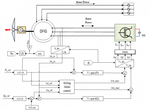
To eliminate the disadvantage of the sliding mode control which is the production of high frequency oscillation caused by its sat(S(x)) switching control, the latter has been replaced by a type-2 fuzzy controller as shown in the following figure:
Figure 10. Fuzzy Sliding Mode control of the active and reactive power
The first input of the fuzzy system is the current error, it is the difference between the reference value and the measured value of currents, and the second input is the error derivative of the latter.
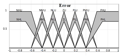
The entries are represented by seven language labels: Negative High (NH), Negative Medium (NM), Negative Low (NL), Zero (Z), Positive Low (PL), Positive Medium (PM), and Positive High (PH). The MFs for the inputs are selected as follows:
Triangular for NM, NL, Z, PL, PM and trapezoidal for NH and PH labels.
The MFs representing the inputs are shown in Figure 11.
Figure 11. Membership for inputs
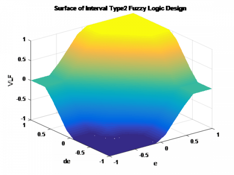
The surface of the controller is shown in Figure 12.
Figure 12. Surface of interval type 2
Table 1. Membership for output
|
Memberships functions |
INTERVAL |
|
HD |
[-1.0, -0.4] |
|
MD |
[-0.6, -0.2] |
|
LD |
[-0.4, 0.0] |
|
Z |
[-0.2, 0.2] |
|
LI |
[ 0.0, 0.4] |
|
MI |
[ 0.2, 0.6] |
|
HI |
[ 0.4, 1.0] |
The output of the fuzzy system is the variation of the attractive control. This output is represented by five language labels: high decrease (HD), Medium decrease (MD), low decrease (LD), Zero (Z), low increase (LI), Medium increase (MI) and high increase (HI). The MFs representing the output are shown in table 1.
We have seven values of error (e) and seven values of change in error (de) then we will have 49 rules to cover all possible inputs. These are often simply written in a table as follows:
Table 2. Rules table of the fuzzy controller
|
E ΔE |
NH |
NM |
NL |
Z |
PL |
PM |
PH |
|
NH |
HD |
HD |
HD |
HD |
MD |
LD |
Z |
|
NM |
HD |
HD |
HD |
MD |
LD |
Z |
LI |
|
NL |
HD |
MD |
MD |
LD |
Z |
LI |
MI |
|
Z |
HD |
MD |
LD |
Z |
LI |
MI |
HI |
|
PL |
MD |
LD |
Z |
LI |
MI |
HI |
HI |
|
PM |
LD |
Z |
LI |
MI |
HI |
HI |
HI |
|
PH |
Z |
LI |
MI |
HI |
HI |
HI |
HI |
The mathematical model of the overall system has been simulated in Matlab-Simulink. The parameters of the wind turbine and the DFIG are given in appendix [6, 17].
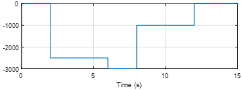
In our simulation, the active power is sent to the electrical grid, while the stator reactive power setpoint will be maintained at zero (Qs=0 VAR) to ensure a unit power factor on the stator.
To check the control laws proposed in this work and to check the decoupling between the active and reactive stator powers (Ps and Qs), we give different instructions with different moments for the power active stator, which are shown in the Figure 10.
The figures presented show the performance of the Sliding Control of a DFIG based on Fuzzy Type-2 Controller applied to a cascade using a two-level inverter connected to the rotor of the DFIG which is pulled by a wind turbine.
In this test, an instruction was given for the active power to be injected into the electrical grid. There is a good follow-up of the instructions for the active power as well as for the reactive power of the stator which is maintained at zero by the real powers delivered by the DFIG. This technique made it possible to obtain a perfect decoupling enters the two components of the stator power.
Figure 13. Profile for the power active stator
Figure 14. Stator voltages
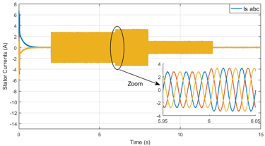
Figure 15. Stator currents and Zoom of the DFIG
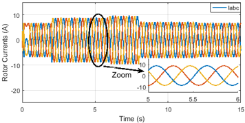
Figure 16. Rotor currents and Zoom of the DFIG
Figure 17. Fuzzy Sliding mode control profile of: (a) Active Power, (b) Reactive power
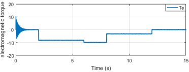
Figure 18. The electromagnetic torque
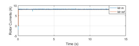
Figure 19. Direct and quadrature rotor currents of the DFIG for F-SMC controller
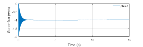
Figure 20. Direct and quadrature stator flux of the DFIG
This work, dedicated to the modeling, simulation and control of a wind energy conversion system by MPPT control for the extraction of the maximum power of the wind turbine, to independently control the active and reactive power we used the sliding mode control based on the fuzzy controller type-2.
The modelling, development and analysis of control laws are presented. These controls are applied to regulate the active and reactive power of the double-fed induction generator to their reference values. According to the simulation results obtained, the proposed controller shows satisfactory dynamic performance, it gives a reduced response stabilization time for the DFIG quantities, it allows a fast response without exceeding and it performs a perfect control with regard to the monitoring of the power setpoints. This article has opened many doors for the future work will be on the use of other types of controllers that will be based on artificial intelligence and hybrid controllers, such as artificial neural network with PI regulator for the control of the DFIG and the implementation of these commands on a real-time simulation system, such as OPAL-RT.
Vsd, Vsq, Vrd, Vrq Stator and rotor voltage components in the d-q reference frame.
Isd , Isq ,Ird , Irq Stator and rotor current components in the d-q reference frame.
Φsd, Φsq, Φrd, Φrq Stator and rotor flux components in the d-q reference frame.
ωs, ωr Stator frequency, rotor rotating speed.
p Number of pole pairs.
Rs, Rr Stator-Rotor resistance.
Ls, Lr Stator and Rotor inductance respectively.
Lm Mutual inductance.
Ps, Qs Active reactive stator power respectively.
Tem Electromagnetic torque.
APPENDIX
Table 3. Rated data of the simulated DFIG
|
Parameters |
definition |
value |
|
Pn Rs Rr Ls Lr M p J f |
Nominal power Stator resistance Rotor resistance Cyclic stator inductance Cyclic rotor inductance Mutual inductance Number of pairs of poles Inertia moment Friction coefficient |
4 KW 1.2 Ω 1.8 Ω 0.1554 H 0.1568 H 0.15 H 2 0.2 kg.m2 0.001 Nm.s |
[1] Blaabjerg, F., Teodorescu, R., Liserre, M., Timbus, A. (2006). Overview of control and grid synchronization for distributed power generation systems. IEEE Transactions on Industrial Electronics, 53(5): 1398-1409. https://doi.org/10.1109/TIE.2006.881997
[2] Abad, G., Lopez, J., Rodriguez, M., Marroyo, L., Iwanski, G. (2011). Doubly fed induction machine.
[3] Errouissi, R., Durra, A.A., Muyeen, S.M., Leng, S., Blaabjerg, F. (2017). Offset-free direct power control of DFIG under continuous-time model predictive control. IEEE Transactions on Power Electronics, 32(3): 2265-2277. https://doi.org/10.1109/TPEL.2016.2557964
[4] Zavadil, R., Miller, N., Ellis, A., Muljadi, E. (2005). Making connections: Wind generation challenges and progress. IEEE Power and Energy Magazine, 3(6): 26-37. https://doi.org/10.1109/MPAE.2005.1524618
[5] Xiong, L., Wang, J., Mi, X., Khan, M.W. (2018). Fractional order sliding mode based direct power control of grid-connected DFI. IEEE Transactions on Power Systems, 33(3): 3087-3096. https://doi.org/10.1109/TPWRS.2017.2761815
[6] Belounis, O., Labar, H. (2017). Fuzzy sliding mode controller of DFIG for wind energy conversion. International Journal of Intelligent Engineering and Systems, 10(2): 163-172. https://doi.org/10.22266/ijies2017.0430.18
[7] Krishnama, R.S., Pillai, G.N. (2016). Design and implementation of type-2 fuzzy logic controller for DFIG-based wind energy systems in distribution networks. IEEE Transactions on Sustainable Energy, 7(1): 345-353.
[8] Djafar, D., Belhamdi, S., Goléa, A. (2018). Speed control of induction motor with broken bars using sliding mode control (SMC) based to on type-2 fuzzy logic controller (T2FLC) . AMSE Journals Advances C, 73(4): 197-201. https://doi.org/10.18280/ama_c.73009
[9] Mendel, J.M., Rajati, M.R. (2014). On computing normalized interval type-2 fuzzy sets. IEEE Transactions on Fuzzy Systems, 22(5): 1335-1340. https://doi.org/10.1109/TFUZZ.2013.2280133
[10] Mendel, J.M. (2014). General type-2 fuzzy logic systems made simple: A tutorial. IEEE Transactions on Fuzzy Systems, 22(5): 1162–1182. https://doi.org/10.1109/TFUZZ.2013.2286414
[11] Ruiz, G., Hagras, H., Pomares, H., Rojas, I., Bustince, H. (2016). Join and meet operations for type-2 fuzzy sets with nonconvex secondary memberships. IEEE Transactions on Fuzzy Systems, 24(4): 1000-1008. https://doi.org/10.1109/TFUZZ.2015.2489242
[12] Miguel, L.D., Santos, H., Sesma-Sara, M., Bedregal, B., Jurio, A., Bustince, H., Hagras, H. (2017). Type-2 fuzzy entropy sets. IEEE Transactions on Fuzzy Systems, 25(4): 993-1005. https://doi.org/10.1109/TFUZZ.2016.2593497
[13] Mendel, J.M., Wu, D. (2017). A new look at type-2 fuzzy sets and type-2 fuzzy logic systems. IEEE Transactions on Fuzzy Systems, 25(3): 725-727. https://doi.org/10.1109/TFUZZ.2016.2543746
[14] Li, R., Jiang, C., Zhu, F., Chen, X. (2016). Traffic flow data forecasting based on interval type-2 fuzzy sets theory. IEEE/CAA Journal of Automatica Sinica, 3(2): 141-148. https://doi.org/10.1109/JAS.2016.7451101
[15] Sun, Z., Wang, N., Srinivasan, D., Bi, Y. (2014). Optimal tunning of type- 2 fuzzy logic power system stabilizer based on differential evolution algorithm. International Journal of Electrical Power & Energy Systems, 62(11): 19-28. https://doi.org/10.1016/j.ijepes.2014.04.022
[16] Hassani, H., Zarei, J., Arefi, M.M., Razavi-Far, R. (2017). Zslices-based general type-2 fuzzy fusion of support vector machines with application to bearing fault detection. IEEE Transactions on Industrial Electronics, 64(9): 7210-7217. https://doi.org/10.1109/TIE.2017.2688963
[17] Melin, P., Gonzalez, C.I., Castro, J.R., Mendoza, O., Castillo, O. (2014). Edge-detection method for image processing based on generalized type-2 fuzzy logic. IEEE Transactions on Fuzzy Systems, 22(6): 1515-1525. https://doi.org/10.1109/TFUZZ.2013.2297159
[18] Rahali, X.O., Zeghlache, S., Benalia, L. (2017). Adaptive field-oriented control using supervisory type-2 fuzzy control for dual star induction machine. International Journal of Intelligent Engineering and Systems, 10(4): 28-40. https://doi.org/10.22266/ijies2017.0831.04
[19] Md, R.I, Guo, Y., Zhu, J.G. (2011). Steady state characteristic simulation of DFIG for wind power system. IEEE Trans. Electrical and Computer Engineering (ICECE), 151-154. https://doi.org/10.1109/ICELCE.2010.5700649
[20] Du, Z., Gu, W. (2009). Aerodynamics analysis of wind power. World Non-Grid-Connected Wind Power and Energy Conference, 1-3: 24-26.
[21] Nunes, M.V.A., Lopes, J.A.P., Zurn, H.H., Bezerra, U.H., Almeida, R.G. (2004). Influence of the variable-speed wind generators in transient stability margin of the conventional generators integrated in electrical grids. IEEE Transactions on Energy Conversion, 19(4): 692-701. https://doi.org/10.1109/TEC.2004.832078
[22] Abdin, E.S., Wilson, X. (2000). Control design and dynamic performance analysis of a wind turbine-induction generator unit. IEEE Transactions on Energy Conversion, 15(1): 91-96. https://doi.org/10.1109/60.849122
[23] Winkelman, J.R., Javid, S.H. (1983). Control design and performance analysis of a 6 MW wind turbine generator. IEEE Transactions on Power Apparatus and Systems, 102(5): 1340-1347. https://doi.org/10.1109/TPAS.1983.318083
[24] Bedouda, K., Ali-rachedi, M., Bahi, T., Lakel, R., Grid, A. (2015). Robust control of doubly fed induction generator for wind turbine under sub-synchronous operation mode. Energy Procedia, 74: 886-899. https://doi.org/10.1016/j.egypro.2015.07.824
[25] Benkahla, M., Taleb, R., Boudjema, Z. (2016). Comparative study of robust control strategies for a dfig-based wind turbine. International Journal of Advanced Computer Science and Applications, 7(2): 455-462. https://doi.org/10.14569/IJACSA.2016.070261
[26] Rouabhi, R., Abdessemed, R., Chouder, A., Djerioui, A. (2015). Power quality enhancement of grid connected doubly-fed induction generator using sliding mode control. International Review of Electrical Engineering, 10(2): 1827-6660.
[27] Müller, S., Deicke, M., De Doncker, R.W. (2002). Doubly fed induction generator systems. IEEE Industry Applications Magazine, 8(3): 26-33. https://doi.org/10.1109/2943.999610
[28] Bounar, N., Boulkroune, A., Boudjema, F. (2014). Adaptive fuzzy control of doubly-fed induction machine. CEAI, 16(2): 98-110.
[29] Lei, Y., Mullane, A., Lightbody, G., Yacamini, R. (2006). Modeling of the wind turbine with a doubly fed induction generator for grid integration studies. IEEE Transactions on Energy Conversion, 21(1): 257-264. https://doi.org/10.1109/TEC.2005.847958
[30] Rahali, H., Zeghlache, S., Benalia, L., Layadi, N. (2018). Sliding mode control based on backstepping approach for a double star induction motor (DSIM). AMSE Journals, Advances C, 73(4): 150-157. https://doi.org/10.18280/ama_c.730404
[31] Merabet, A., Eshaft, H., Tanvir, A.A. (2018). Power-current controller based sliding mode control for DFIG-wind energy conversion system. IET Renewable Power Generation, 12(10): 1155-1163.
[32] Zadeh, L.A. (1965). Fuzzy sets. Information and Control, 8(3): 338-353. https://doi.org/10.1016/S0019-9958(65)90241-X
[33] Zadeh, L.A. (1975). The concept of a linguistic variable and its application to approximate reasoning-I. Information Sciences, 8(3): 199-249. https://doi.org/10.1016/0020-0255(75)90036-5
[34] Mendel, J.M. (2001). Uncertain rule-based fuzzy logic systems: Introduction and new directions. Springer, Germany.
[35] Mndel, J.M. (2017). Uncertain rule-based fuzzy systems: Introduction and new directions. Springer, Germany.