Aicha Kharouati* | Nasr Eddine Debbache
OPEN ACCESS
We know that different intelligent instruments play an important role in the evolution of various industrial systems dependability. This role is mainly due to the additional functionality of the compensation, validation, self-diagnosis and self-configuration functions, combined with appropriate means of communication. For this reason, this article presents an in-depth study of the contribution of intelligent instruments for improving mechatronic system dependability. In this paper, we note that the indicators taken into account as an evaluation criterion is the probability of dangerous failure (PFD) and the probability of safe failures (PFS). To carry out this study, three modeling approaches of functional and dysfunctional behavior of studied system in the classical case and intelligently face, namely: fault tree, reliability diagram and Stochastic Petri Network have been adopted. In first time, it is interesting to determine the most appropriate approach to modeling the studied case study. We note that, the treated parameters in this study are simulation software tool used in this study is GRIF (Interactive Graphics for Reliability): reliability, availability and two security indicators PFD and PFS. The simulation software tool used in this study is GRIF (Interactive Graphics for Reliability).
dependability, intelligent instrument, probability of dangerous failures, probability of safe failure, stochastic petri network
Nowadays, different dependability studies should consider diversity faults issues (physical, human...) [1], diversity of relationships between faults and failures (layers of jumps and subsystems limits interactions between faults) and defining faults (dynamic changing specifications) [2]. We recall that assessing the reliability of a system involves analyzing component failures to estimate their impact on the service provided by the system [3].
We are particularly interested in the derived standard IEC 61511 [5] which is applicable to the process industry sector, IEC 61511 Functional safety, Safety Instrumented Systems (SISs) for the process industry sector, International Electrotechnical Commission (IEC) has been developed as a process sector implementation of the generic standard IEC 61508 Functional safety of electrical/electronic/programmable electronic safety-related systems, International Electrotechnical Commission (IEC) [1-16]. This standard is primarily concerned with Safety Instrumented Systems (SISs) for the process industry sector [16]. SISs are defined as the systems or sub-systems responsible for safety-related sensing elements to determine an emergency situation, safety-related logic solvers to determine what action to take and safety-related final elements to implement the action [16].
Considering the IEC 61508 specifies two security indicators for programmable electronic systems dedicated to safety applications. IEC 61508 Functional safety of Electrical/Electronic/Programmable Electronic (E/E/PE) safety related systems, [4]. This set of standards becomes the benchmark for the development, implementation and deployment of security systems [9]. It is important to note that the two indicators of dangerous and safe failure probability (PFD & PFS) used to assess the safety of an industrial system relate to two failure modes mentioned in this standard [12]. This is a mode or situation of dangerous failures and the way of safe faults represented respectively by the probability of dangerous failure (PFD) and the probability of safe failure (PFS) [11, 10, 17].
To recall, the dangerous failure is a complicated situation with a capacity to put the safety instrumented system unable to perform a safety function [18]. A dangerous failure is a failure which tends to inhibit this function in case of request emanating from the watched process which will be then in a dangerous state [14].
On another side, the safe failure has not the potential to put the safety instrumented system in a dangerous state [18]. A safe failure is an inconvenient failure which tends to anticipate the release of the same function (in the absence of any request) by leading actually the process watched in a safe state [14].
If we project this into the industrial world, it is known that dangerous failures put the system in a complicated state of failure. It is interesting to note that in the case of dangerous failures cases, the safety function is no longer executed because one or more components are faulty [3-10, 17-19]. To avoid the situation of dangerous failure, the use of intelligent instruments seems appropriate. These instruments have the main purpose of turning dangerous failures in safe failures [18]. The problem is to quantify the contribution of the use of the intelligent instruments in the safety loops in compliance with related standards. In safety systems many studies were developed for dependability evaluation.
For recall, dependability is a generic concept. These main concepts are: reliability, availability, maintainability and safety [1, 7-8].
These approaches ignore the use of intelligent instruments. The dependability evaluation of intelligent instruments is a difficult task and can concern two approaches: a static approach and a dynamic approach which takes into account the progressive evolution of system states and functioning modes [15-16].
In the present paper, we focus on the contribution of these instruments like sensors, intelligent actuators that replace conventional sensors actuators in mechatronic systems. The quantitative analysis for analysing the dependability of mechatronic systems is based to the results of qualitative analysis [20].
The main methods discussed in this work during the reliability analysis are the fault tree, the reliability diagram and the Stochastic Petri Network.
We note that the set of the treated dependability parameters are: the reliability, availability and safety of the two indicators, namely the probability of dangerous failure and the probability of safe failures. The simulation software tool used is GRIF (Interactive Graphics for Reliability) [7].
It is known that an intelligent instrument, whether a sensor or an actuator, is a device that provides additional functionality. These instruments combine data acquisition, internal and external system processing and provide compensation functions (such as validation, self-diagnosis and self-configuration) combined with appropriate means of communication (for more details, the reader is invited to consult the study of [1-19].
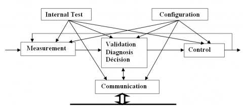
The functional structure of an intelligent instrument is shown in Figure 1:
Figure 1. Functional structure of an intelligent instrument [1-17, 19]
The involvement of the smart instrument in the system involves, among other actions, participation in the alarm security system by providing opportunities to control the system by integrating control functions [16].
The intelligent instruments offer the possibility of a local processing of the information which is distributed on the various entities and thus allowing a distribution of the execution of the tasks in the context of a distributed control [16].
We can observe that the diagram presented by Figure 1 shows the functional architecture of intelligent instruments presented by a classic chain of Measurement-Decision-Action.
The main feature that characterizes smart instruments is represented by the core validation, diagnosis and decision. This latter is the heart of a smart instrument. This feature relates to the environmental condition’s correction, validation, implementation of diagnosis functions and decision making [3-13, 17-19].
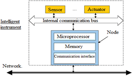
The hardware structure of an intelligent instrument is shown in figure 2.
It is worth notising note that an intelligent instrument is composed of several sensors or actuators connected to a node via an internal bus. This instrument can be composed only of sensors, actuators or both (for more details about point this, the reader is invited to consult [3-10, 17-19].
On another side, a node is a set of components, the main ones are.
- Microprocessor: Can perform calculations
- Memory (ROM or EPROM, RAM),
-The communication interface: This allows managing the reception or transmission of data over the network [18].
Figure 2. Material Structure of an intelligent instrument [3-13, 17-19]
After recalling the definition and the various components of an intelligent instrument, we proceed now to present the studied case in this paper with its various modeling techniques.
The system study is mechatronic systems concerns the volume regulating both tanks passive redundancy using a single tank at a time. This system is shown schematically in the figure 3.
Figure 3 shows the frame of such a system, consisting of a logic solver, two pumps: pump1and pump 2, three solenoid valves EV1, EV2 and EV3 (relief valve), two sensors volume of two tanks (tank 1 and tank 2) regulated in volume measure and a third drain [8].
Both regulated tanks supply users in a predefined need (function of time) and the purpose of the logic solver is dedicated to keep the volume between two predefined values Vmin and Vmax [20].
To do this, the logic solver has the information provided by the two sensors and controls the valves EV1 and EV2 main. If the solenoid valve EV1 or EV2 fail, the logic solver can still act on the volume of liquid in the tank through the relief valve (EV3) for emptying, as it remains operational. If the solenoid valve EV3 also fails, this leads to the overflow tank. In the sake of simplicity, we assume that:
-Only three solenoid valves (EV1, EV2, EV3) and the two sensors 1 and 2 are subject to failure [8].
-Solenoid valves EV1 and EV2 provided for feeding the respective tanks, the opening may be blocked,
-The failure of the solenoid valve EV3 (off) leads the system to a state of dangerous failure (overflow tank).
The tank 1worksas follows: when the volume in the tank is equal to Vmax, the logic solver is the option of closing the solenoid valve EV1. If the solenoid valve EV1 is faulty and the volume in the tank exceeds the supper limit of safety (V1L), logic solver executes the opening of the solenoid valve EV3 to the emptying of the tank1. If the two solenoid valves EV1 and EV3 fail and the volume in the tank exceeds the safety threshold (V1S), then the tank 1 overflows [20]. The same principle of the tank 2’s operation.
The safety function is performed while protecting the system from going into a state of overflow tank, thus reducing the dangerous failures in the system.
Figure 3. Volume control system of two tanks passive redundancy
4.1 Modeling process
The main methods discussed in this work during an analysis of the dependability are:
Fault tree, reliability diagram and stochastic Petri network.
(1) Modeling by fault tree
Figure.4 illustrates the classic tree failures on operating conditions of the system studied under GRIF.
Figure 4. Tree classic system failures in two tanks
The level control system of Figure 3 is governed by the logical expression R associated with the fault tree of Figure 4 and defined by:
R = (((DF1 OR DF2) AND (DF3 OR DF4)) OR DF5)
Where:
DF1, DF2, DF3, DF4 and DF5 are respectively:
DF1: failure 1, DF2: failure 2, DF3: failures 3, DF4: failure 4, DF5: failure 5.
OR and AND are Logical functions.
(2) Modeling by reliability block diagram (RBD)
It is known that the reliability method is a logical block of diagram representation of system operation. The system components are modeled by blocks connected by arcs in the sense that there is a path in the graph between the input and the output in order to ensure that system will be functional [3].
Figure 5 shows the modeling of the system by reliability bloc diagram in GRIF. The model is equivalent to the model of the fault tree of Figure 4.
Figure 5. Diagram of system reliability in two tanks
(3) Modeling by stochastic petri network
To model random behavior, discrete or content, which is the case in the mechatronic system [8]. Mechatronic systems are hybrid systems include both continuous and discrete variables. Continuous dynamics is usually provided by differential and algebraic while the discrete part is modeled by automata or transitions to states.
The systems mechatronics is reliable systems and protect in the purpose time but after several uses in long time (10000 hours) the reliability and the availability of these systems are decreased in that case replaces the elements of the classic system (sensor, actuator) by intelligent instruments (sensor, actuator) thus one result a system mechatronics intelligent safe and more reliable than the classic system.
The Stochastic Petri Network tool is best suited. In the present case of study, we perform the injection of random failures.
Model of sensor. There are two models of the sensor.
Model of classic sensor. The model classic sensor is described by Figure 6.
In this model, the places P1 and P2 respectively represent the operating state and the malfunction of the sensor. Seats P3 to P5 represent the sensor fault [21] qualification part in a hazardous state or P6 (Tc) represents the test state of the sensor by the logic solver.
The model of the actuator is equivalent to the sensor model of figure 6, but each with its own settings. The failure rates of each element (sensor and actuator) [21] are: lambda-sensor (λS) is equal to 6e-6 h-1 and lambda-actuator (λa) is equal to 9e-6 h-6 [6].
Figure 6. Model of classic sensor
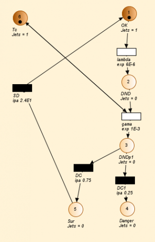
Model of intelligent sensor. The model intelligent sensor is described by Figure 7. The functional part is respectively described by the set of places and transitions from P1 to P6 and T1 to T9. The presence of the token on the left side represents the sensor performance.
Figure 7. The intelligent sensor model
For dysfunctional part, must ensure that the token is removed from the functional part where it is when the system goes down safe or danger.
Where: Pi are the places, Tj are the transitions, i is number of places, j number of transitions.
In this model of the sensor, a number of failures are specified. It is safe failure [21] (Safe Place) and dangerous failures (Danger place). A coverage rate of diagnosis DC is represented by the transition.
IEC 61508 defined the diagnostic coverage DC as the ratio between the rate of detected dangerous failures (a diagnostic test) and the total rate of dangerous failures (detected and undetected) [17]. This rate is represented by the following Eq. (1) [17].
$DC=\frac{\sum_{λ_{DD}}}{\sum_{λ_{dangerous}}}$ (1)
The proportional relationship between safe and dangerous failures is given by the Eq. (2):
DC1=1-DC (2)
The higher of this rate is important, greater confidence in the safety instrumented system that safe conditions prevail in relation to dangerous situations on the occurrence of failures.
After the occurrence of a safe failure, there is the possibility to restore the system by crossing the deterministic transition (SD) whose duration is equal to the time required for complete system recovery. The presence of a mark in the P6 space allows a self-test sensor locally managed. The undetected failures (DND) can be described as safe or dangerous after running the self-test [4-6, 17-19].
The model of the intelligent actuator is equivalent to the model intelligent sensor of Figure 7, but each with its own settings. The failure rates [21] of each element (sensor and actuator) are: lambda-sensor (λS) is equal to 6e-6 h-1 and lambda-actuator (λa) is equal to 9e-6 h-1 [4-6, 17-19].
Model of the logic solver. The model of the logic solver of Figure 8 shows a representation of two parts, one functional and another dysfunctional.
The functional part is described by a set of places and transitions from P1 to P5 respectively and T1 to T7. Cyclically, the logic solver generates its own self-test and self-test of sensor and actuator.
The presence of a token in places P3, P4 or P5 allows one of the aforementioned devices according to a policy managed by the logic solver it self-tests. Self-tests of the various devices are managed locally following a test policy of allocating the same amount of test for different devices and start the test sensor (Tc) and the actuator (Tv) and finally the logic solver (Ta).
For dysfunctional part, must ensure that the token is removed from the functional part where it is when the system goes down safe or danger. The failure rate of the logic solver lambda-logic solver (λl) is equal to 2e-5 h-1 [6]. The logic solver can also be restored in case of safe failure [6].
Figure 8. Model logic solver
Model of tank. The classical model of tank 1 is described in Figure 9. The model of the tank 2 is identical to the model of tank 1. Realized for an intelligent system the classical elements (sensors and actuators (valves)) are replaced by smart sensors and actuators.
In this model, the places P1 and P2 respectively represent the closed state and the opening of the solenoid valve EV1 of the tank 1. The place P3 represents the state of the filling of the water in the tank 1. The places P4, P5 represents respectively the state of good functioning and of failure of the solenoid valve EV1. Places P11 to P15 represent the fault qualification part of the solenoid valve EV1 in a danger state or on.
The places P7 and P8 respectively represent the closed state and the opening of the solenoid EV3 of the tank 1, the places P7, P21 respectively represent the state of operation and failure of the solenoid valve EV 3, Position P9 represents the emptying state of the tank 1. The places P16 to P20 represent the failure qualification part of the solenoid valve EV3 in a danger state or in the place P6 represents the overflow state of the tank 1.
Where: Vmax=100, V1L=110, V1S=120.
The modeling of the classical system is equivalent to linking the classical models of the elements of the system between them: the automaton, the two level sensors, the two solenoid valves, the two tanks according to figure 3.In the case of the intelligent system modeling Is the same but replaces the classic models by the intelligent models of the system elements study.
Figure 9. Model of tank 1
The purpose of the proposed simulation is to observe the behavior of the device according to the conventional structure with structure and intelligence. The approach of stochastic Petri nets (SPNs) are then used to model the behavior of the system because we have replaced models of sensors and actuators (valves) by conventional intelligent models. The software simulation tool GRIF (Interactive Graphics for Reliability), adapted for the study of the reliability and availability with two safety indicators PFD and PFS was used. The coverage diagnosis in this example DC is equal to 75% for all devices (sensor, logic solver and actuator) [6]. To assess the contribution of intelligent systems, we put the system in classical and intelligent situation caused a failure. The injection of a failure in the two situations (classic and intelligent) and for the three elements considered (sensor, actuator and logic solver). This results in the crossing of the transition lambda_logic solver for the logic solver, for example. The dysfunctional part of the logic solver is then shown in the right of Figure 8.
Where the analytical methods used are:
5.1 For the availability
From the simulation results of the system model, we consider the availability according to the following ratio:
$Availability(\%)=\frac{residence time(h)}{period of history(h)}$
The residence time in the place (12) corresponding to (OK_sensor) of Figure 7 it is the same to the actuator. The residence time in the place (6) corresponding to (OK_logic solver) of Figure 8 [6].
The availability calculation is done by the following Eq. (3):
$A(t)= \frac{μ}{λ+μ}+ \frac{λ}{λ+μ} e^{(-(λ+μ)t}$ (3)
where: t is the time in hour, λ is the failure rate [22] and µ is the repair rate.
5.2 For the reliability
DH = history of hours (h),
MTTF = time until the first failure in hours (h).
The calculation of the value of MTTF example in the place (12) corresponding to (OK_sensor) in Figure 7, is realized by the following relation in Eq. (4)
MTTF=DH-time stay in place (12) (4)
From the value of the MTTF, we can easily deduce the failure rate λ which is expressed by Eq. (5):
λ (h-1) =1/MTTF (h) (5)
where the reliability can be inferred from the following relationship in Eq. (6):
R(t)=e_λt (6)
If the system has n components mounted in parallel, the reliability is expressed by Eq. (7):
$R(t)=1-\prod\nolimits_{i=1}^n(1-R_(i)(t))$ (7)
If the n components are in series, the resulting reliability becomes Eq. (8):
$R(t)=\prod\nolimits_{i=1}^nR_i(t)$ (8)
where: t is the time in hour, λ is the failure rate.
The values been of PFD and PFS of the classic system and with intelligence are respectively given onto the Table 1 and the Table 2.
Table 1. PFD and PFS for a classic system
|
Time(h) |
PFD (%) |
PFS (%) |
|
1000 |
0.521×10⁻² |
1.48×10⁻² |
|
4380 |
1. 65 ×10-2 |
2. 81 ×10-2 |
|
5000 |
1. 85 ×10-2 |
0.425 ×10⁻¹ |
|
8760 |
0.221 ×10⁻¹ |
0.615 ×10⁻¹ |
|
10000 |
0.382 ×10⁻¹ |
0.925 ×10⁻¹ |
Table 2. PFD and PFS for an intelligent system
|
Time(h) |
PFD (%) |
PFS (%) |
|
1000 |
0.0112 ×10⁻² |
1.91 ×10⁻² |
|
4380 |
0.0172 ×10⁻² |
8.52 ×10⁻² |
|
5000 |
0.0191×10⁻² |
1.31 ×10⁻¹ |
|
8760 |
0.025 ×10⁻¹ |
1.72 ×10⁻¹ |
|
10000 |
0.125 ×10⁻¹ |
2.25 ×10⁻¹ |
The simulation results are shown in Figure 10, Figure 11 and Figure 12:
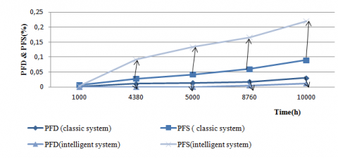
Figure 10. Evolution of the two safety indicators PFD and PFS system over time
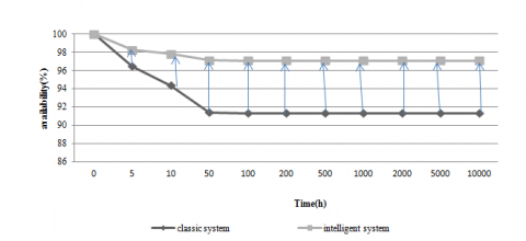
Figure 11. Evolution of system availability over time
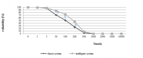
Figure 12. Evolution of system reliability over time
The curve in Figure 10 shows the evolution of two main performance metrics in safety PFD and PFS for a period of 10000 hours (for accurate results). This is a little greater than one year (8670 hours). The two curves indicate exponential speeds. We note a decrease in the value of the PFD and an increase in the value of the PFS compared to the values of the conventional system because of dangerous failures become safe failures.
We can deduce that the conversion of the probability of dangerous failures (PFD) in probability of safe failure (PFS) can be expressed by the effect of the functionality self-diagnostic of an intelligent instrument. Self-diagnosis is the ability of an instrument to carry out the assessment of its condition and diagnose the possibly malfunction item.
The Figure 11 and Figure 12 illustrate the temporal evolution of the availability and reliability of the system to study classical and intelligence for a period of 10000 hours which is a little more than one year (8670 hours). Then, we remark an improvement in both parameters (availability and reliability) for distributed intelligence system.
Thus from the use of the intelligent instruments we result a intelligent méchatronic system available and more reliable.
The authors would like to gratefully acknowledge the Laboratory of Automatic and Signals Annaba (LASA), Badji Mokhtar University, P.O. Box 12, Annaba 23000, Algeria.
|
A(t) AND DF1 DF2 DF3 DF4 DF5 DC DND DH MTTF OR Pi R(t) SD Ta Tc Tv Ti t Vmin Vmax V1L V1S |
the availability % Logical functions failure 1 failure 2 failure 3 failure 4 failure 5 the diagnostic coverage the undetected failures history of hours h time until the first failure in hours h Logical functions places the reliability % the deterministic transition the test state of the logic solver the test state of the sensor the test state of the actuator transitions the time h minimum volume L maximum volume L upper limit of safety of the volume in the tank L the safety threshold of the volume in the tank L |
|
|
Greek symbols |
||
|
λ |
the failure rate in h-1 |
|
|
µ λDD λ dangerous λS λa λl ∑ ∏ Subscripts GRIF IEC PFD PFS SPNs SISs |
the repair rate in h-1. the rate of detected dangerous failures the rate of dangerous failures (detected and undetected) the failure rate of the sensor h-1 the failure rate of the actuator h-1 the failure rate of the logic solver h-1 n-ary summation n-ary product
Interactive Graphics for Reliability International Electrotechnical Commission probability of dangerous failures probability of safe failures Stochastic Petri Nets safety instrumented systems |
|
[1] Megdiche M. (2004). Safe operation of distribution networks in the presence of decentralized production. Ph.D. Institut national polytechnique de Grenoble.
[2] Logiaco S. (1999). Etude de sûreté des installations électriques. Cahier technique. Collection Schneider Technique.
[3] Cabau E. (1999). Introduction à la conception de la sûreté. Cahier technique Schneider Electric.
[4] IEC 61508 (1998). Functional safety of Electrical/Electronic/Programmable Electronic (E/E/PE)-safety related systems. International Electrotechnical Commission (IEC). https://www.iec.ch/functionalsafety/standards/page2.htm
[5] IEC 61511 (2000). Functional safety- Safety Instrumented Systems for the process industry sector. International Electrotechnical Commission (IEC). https://literature.rockwellautomation.com/idc/groups/literature/documents/rm/safebk-rm003_-en-p.pdf
[6] Kharouati A, Menasria Y, Debbache ND. (2014). Use of intelligent instruments for the security functions of a system. Proceedings of Third International Conference on Industrial Engineering and Manufacturing ICIEM’14. Batna University, Algeria, 195-200.
[7] Boumelita D, Ouerdachi L, Debbache NE. (2018). Contribution to study of the dependability of a drinking water system. Journal of Water and Land Development 38(1): 11-18. https://doi.org/10.2478/jwld-2018-0037
[8] Khalfaoui S. (2003). A method for deriving feared scenarios for dependability evaluation of automotive mechatronic systems. Ph.D. Automatique-Robotique. Institut national polytechnique de Toulouse.
[9] Thuy LEN, Adjadi A, Chaumette S, Bouchet S, Valérie de Dainous. (2008). Evaluation des performances des Barrières Techniques de Sécurité. Rapport d’étude n° dra-08-95403-01561B (DCE DRA-73), Evaluation des Barrières Techniques de Sécurité, Ω 10.
[10] Mkhida A. (2008). Validation deficiency of an intelligent sensor and incidence on the performance of the safety loop. 17th Congress of Control of Risks and Dependability, La Rochelle, France, pp. 1-9.
[11] Mkhida A. (2008). Impact de l’utilisation d’un réseau de communication sur les performances en sécurité d’un système instrumente de sécurité. 7e Conférence Internationale de Modélisation et Simulation - MOSIM’08 – Paris, France, pp. 1-8.
[12] Sallak M, Aubry JF. (2008). Optimal design of safety instrumented systems under uncertainty. 16th Congress of Risk Management and Functional Safety-Communication 6B-2, Avignon 1-8.
[13] Brissaud F, Charpentier D, Barros A, Bérenguer C. (2008). Intelligent sensors: new technologies and new dependability issues. 16th Congress of Control of Risks and Dependability, France, pp. 1-8. https://doi.org/10.3182/20090603-3-RU-2001.0129
[14] Innal F, Haddad S, Chebila M, Bahmed L. (2014). Optimisation des Architectures des Systèmes Instrumentés de Sécurité à l’aide des Algorithmes Génétiques Proceedings of Third International Conference on Industrial Engineering and Manufacturing ICIEM’14. Batna University, Algeria, pp. 603-609.
[15] Mkhida A, Thiriet JM, Aubry JF. (2008). Toward an intelligent distributed safety instrumented systems dependability evaluation. 17t J-M. h IFAC World Congress (IFAC'08) Seoul 14(2): 3586-3591. https://doi.org/10.3182/20080706-5-KR-1001.00606
[16] Mkhida A, Thiriet JM, Aubry JF. (2014). Integration of intelligent sensors in safety instrumented systems (SIS). Process Safety and Environmental Protection 92(2): 142-149. http://dx.doi.org/10.1016/j.psep.2013.01.001
[17] Mechri W. (2011). Evaluation of the performance of systems with inaccurate parameters. Ph.D.
[18] Mkhida A. (2008). Contribution to the evaluation of the dependability of safety instrumented systems incorporating intelligence. Ph. D formation in Automatic, Nancy University.
[19] Clarhaut J. (2009). Accounting for failure sequences for design automation systems Application to piggyback. Ph.D. Automatic, Computer Engineering, Signal Processing and Images Science and Technology, Science and Technology of Lille Univercity.
[20] Boucerredj L, Debbache NE. (2007). Modelling of a hybrid system through differential predicate transition Petri nets model and proof tree. Aircraft Engineering and Aerospace Technology, an International Journal 3(79): 261-267. https://doi.org/10.1108/00022660710743868
[21] Boumaiza A, Arbaoui F, Saidi ML. (2018). Intelligent condition monitoring of variable speed wind energy conversion systems based on decentralized sliding mode observer. Advances in Modelling and Analysis C (73)2: 37-44. https://doi.org/10.18280/ama_c.730202