Tohid Adibi
OPEN ACCESS
In this paper, the influence of icy boundary on the drag force is studied experimentally. For this purpose, at first, the drag force on NACA0015 airfoil is measured in a subsonic wind tunnel. The span of airfoil is 15 cm and its chord are 20 cm and the section of airfoil for experiments is 300×450 mm. Then, a cast is designed to produce icy airfoil with the same dimensions of aforementioned airfoil. The drag force of icy airfoil is measured in the same wind tunnel, too. Polyamid is used to make the cast. The results show that the drag force on the icy airfoil is up to 40 % less than non-icy one. This reduction is lower for smaller attack angles. Delayed boundary layer separation is the main reason for decrease in drag force. Sublimation of icy airfoil produces the secondary flow accompanying with a new boundary layer under the primary one. The secondary boundary layer is another reason for reduction of drag force. Experiments are conducted at different attack angles between and The Reynolds numbers are between 105 and 2.5×10⁵. The accuracy of experimental instruments is considered and the results are obtained after numerical error analysis.
drag force reduction, NACA0015 airfoil, icy airfoil, separation, attack angle
Fluid flow over solid bodies is very important in several engineering fields such as mechanical engineering, marine engineering, aerodynamics and etc. To design solid bodies as airplane and ship, the calculation of forces including both the drag and lift forces acting on these bodies is crucial. The governing equations are complicated and in the most problems, do not have any exact analytical solutions. Numerical and experimental methods are alternative approaches. In this research, an experimental method is employed to measure the drag force on solid bodies.
Zhou et al. [1] investigated the flow around a smooth cylinder and a longitudinally grooved cylinder at Reynolds numbers ranging from 7.4×10³ to 1.8×10⁴ experimentally. This paper meant to found an improved understanding of effects of the grooved surface on the drag coefficient and the flow characteristics of cylinder. Gylys et al. [2] presented an analysis of the drag force decrease through the hot spherical and cylindrical bodies movement in the water in contrast with the movement of cold bodies. Effect of 2-phase water–vapor flow on the drag force was studied both experimentally and numerically. The initial consequences of study showed an adequate decrease of drag force for the hot body in relationship to the cold body due to vapor existence. Niknafs and Rad [3] presented a towing tank based experimental study on drag forces for different Reynolds numbers of a special underwater model. This paper discovered drag force and coefficient in a diverse flow direction over the model. Obtained experimental outcomes were clarified. Khaled et al. [4] concentrated on a parametric study of trends in aerodynamic forces. They described aerodynamic force measurements carried out on a basic vehicle model. Experiments were done in a wind tunnel for changed airflow configurations in order to separate the parameters to approve others earlier suspected. Nakamura and Igarashi [5] reached a drag decrease for a round cylinder exposed to the cross-flow by attaching cylindrical rings along its span at an interval of numerous diameters. The Reynolds number based on the diameter of the cylinder ranged from 3000 to 38000 for the tests. The adding of the rings decreased the drag force by 15 % for Red⩾20 000, even though the projected area enlarged. Polidori et al. [6] did skin-friction drag force analysis in the underwater swimming. From a simplified model in a variety of pool temperatures, it was confirmed that whatever the swimming speeds, a 5.3 % discount in the skin-friction drag would happen with growing average boundary-layer.
Mirzaei et al. [7] studied the characteristics of separated bubbles and unsteady features of flow fields around a glaze-iced airfoil. The study was did using both experimental and numerical methods. The experimental measurements were carried out using the hot-wire anemometry at Reynolds number of 0.5×10⁶ and attack angle ranging from 0° to 6°. Koomullil et al. [8] offered a new plan for simulating the flow around iced airfoils. Two different tactics were applied to generate qualified grids over the iced airfoil. Both grids can be categorized as generalized grids since multiple element types were working in each.
Tsao and Rothmayer [9] advanced a viscous–inviscid interaction triple-deck building to define the thermo-mechanical interaction of an air boundary layer with ice sheets and liquid films. Linear stability outcomes were compared with nonlinear triple-deck calculations, and a number of nonlinear simulations of air–water–ice interactions were presented. Kornilov [10, 11] considered the drag of an axisymmetric body of revolution in the incompressible flow experimentally. In other work, he organized some experiments to study the possibility of reducing the net drag force of a flat plate with the usage of streamwise-oriented vertical elements mounted normal to the surface in the incompressible turbulent flow.
Leontiev and Milman [12] considered the influence of condensing steam flow parameters. The total pressure reduction of steam was upper for the counter-flow. The pressure rduction was calculated with diverse computation schemes. Semenov [13] offered the chief principles and approaches of developing the single-layer monolithic compliant coatings for the turbulent drag force reduction. Rabani et al. [14] studied experimentally and numerically the effect of the crosswind and wagon numbers to the aerodynamic characteristics. Three dimensional incompressible turbulent airflow has been considered for numerical simulation. The consequences presented that the variation of the longitudinal force coefficient (LFC) and side force coefficient (SFC) in the medium wagons is similar. Majumder et al. [15] did an experimental study of the turbulent fluid flow through a rectangular diffuser. Their expements are done for incompressible 3D turbulent flow with Re=6.2 × 10⁴. Fouad et al. [16] studied on the effect of solution velocity in the absence and presence of drag- reducing polymer on the rate of diffusion controlled corrosion experimentally. Natarajan et al. [17] determined the optimum shape for fore body in inviscid supersonic flow with an attached shock constraint numerically.
There are a lot of ways to reduce the drag. In this paper, the influence of icy boundary on the drag force was investigated experimentally.
2.1 Wind tunnel
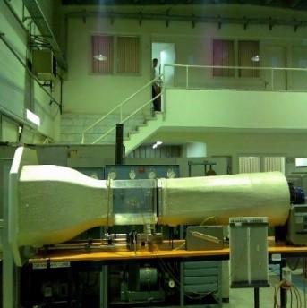
A subsonic wind tunnel is used to measure the drag force on the solid bodies. This tunnel has been shown in Figure 1. The convergent and divergent sections of this tunnel is fabricated from fiber glass and its shape is a hexagon with 300 mm sides. A 5-fins fan is located in the exit of tunnel and is rotated with a motor to produce pressure difference. This pressure difference produced air flow. Wind tunnel properties are displayed in Table 1.
Figure 1. Subsonic wind tunnel which is used to measure the drag force on solid bodies
Table 1. Wind tunnel properties
|
wide |
0.8 m |
Electrical power supply |
240 V, 50 Hz |
|
length |
2.98 m |
Range of drag force |
2.5 N |
|
Test section |
300×450 mm |
Measurement accuracy |
0.01 N |
Monometers are used to measure the total and static pressures. Water is used as manometer's liquid. The difference between total and static pressures is calculated from Eq. (1).
${{P}_{total}}-{{P}_{static}}=\,\,\rho g\Delta h$ (1)
The velocity of air flow is calculated from dynamic pressure with
${{P}_{total}}-{{P}_{static}}=\,\,{{P}_{dynamic}}\,\,=\,\,\frac{1}{2}\rho {{V}^{2}}\to V\,=\,\sqrt{\frac{2{{\rho }_{water}}g\Delta h}{{{\rho }_{air}}}}$ (2)
Air density is obtained by
${{\rho }_{air}}\,=\,\frac{{{P}_{air}}}{{{R}_{air}}{{T}_{air}}}$ (3)
2.2 Fabricating non-icy and icy airfoils
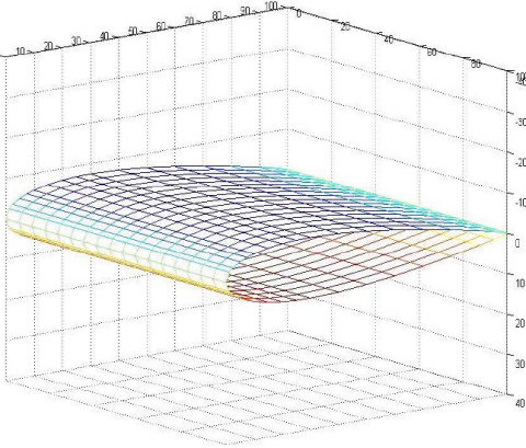
In the next step, one needs to design and make an icy-boundary solid and non-icy boundary solid. So, a NACA0015 airfoil is fabricated with 15 cm span and 20 cm chord. The three and two dimensional shapes of this airfoil are illustrated in Figure 2.
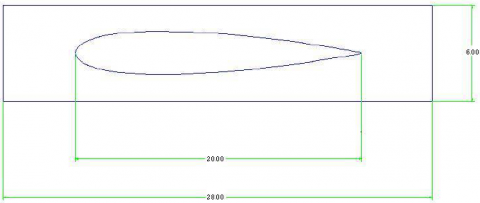
Then, a cast is made to produce an icy-boundary airfoil with the same dimensions. In order to protect the cast from cracking induced by freezing, the material chosen for the cast should be soft and flexible. This material should not be very flexible because more flexibility leads to mismatch between the icy model and the non-icy one. So, polyamid is selected as the appropriate material for the cast. To produce icy airfoil, mentioned cast is filled with water and then water in cast is frozen in a refrigerator. So, icy airfoil is exited from the cast and is located in a wind tunnel. The three and two dimensional shapes of mentioned cast are shown in Figure 3.
Figure 2. Three and two dimensional shapes of non-icy airfoil
Figure 3. Three and two dimensional shapes of cast
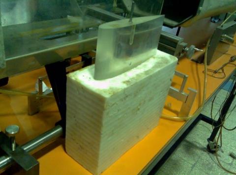
The non-icy airfoil and the cast are depicted in Figure 4.
Figure 4. Model and cast which are fabricated to form an icy-airfoil
2.3 Experimental methodology
2.3.1 Experiments on the non-icy model
After making the model, the experiments were conducted in the following steps:
Assembling the non-icy airfoil in the wind tunnel.
Adjusting the attack angle on a specific attack angle.
Balancing the initial forces.
Starting the experiments and changing the velocity
Changing the attack angle and repeating the steps above.
2.3.2 The experiments on icy airfoil
At first, the water is filled inside the cast up to calculated height and then it is put inside a refrigerator. The steps aforementioned for a non-icy airfoil are conducted for the icy model. The Reynolds number of flow is defined as
$\operatorname{Re}=\frac{{{\rho }_{air}}Vt}{{{\mu }_{air}}}$ (4)
In the above equation, t is the thickness of airfoil. In all numerical calculations, error analysis is done to determine the significant digits. For example, to determine the accuracy of calculated Reynolds number, this equation is used
$\begin{align} & \left| \operatorname{Re}-{{\operatorname{Re}}^{*}} \right|\le \left| \frac{\partial \operatorname{Re}}{\partial V} \right|*\left| V-{{V}^{*}} \right|+\,\left| \frac{\partial \operatorname{Re}}{\partial {{\rho }_{air}}} \right|* \\ & \left| {{\rho }_{air}}-\rho _{air}^{*} \right|+\,\left| \frac{\partial V}{\partial D} \right|*\left| t-{{t}^{*}} \right|+\,\left| \frac{\partial \operatorname{Re}}{\partial {{\mu }_{air}}} \right|*\left| {{\mu }_{air}}-\mu _{air}^{*} \right| \\\end{align}$ (5)
In the above equation "*" is used for real value of quantity. Other quantity is obtained with experiments or with numerical calculations. According to accuracy of the experimental instruments, one has
$\left| t-{{t}^{*}} \right|\le 0.5*{{10}^{-4}}$ (6)
$\left| {{\mu }_{air}}-\mu _{air}^{*} \right|\le 0.5*{{10}^{-7}}$ (7)
And after an error analysis for density and velocity, one has
$\left| {{\rho }_{air}}-\rho _{air}^{*} \right|=\text{0}\text{.007705898}$ (8)
$\left| V-{{V}^{*}} \right|\le \text{0}\text{.000769097}$ (9)
So,
$\begin{align} & \left| \operatorname{Re}-{{\operatorname{Re}}^{*}} \right|\le \left| \frac{1.0*0.200}{184*{{10}^{-7}}} \right|*\left| \text{0}\text{.000763398} \right| \\ & +\left| \frac{\text{23}\text{.15}*0.200}{184*{{10}^{-7}}} \right|*\left| \text{0}\text{.007705898} \right|+ \\\end{align}$
$\begin{align} & +\left| \frac{1.0*\text{23}\text{.15}}{184*{{10}^{-7}}} \right|*\left| 0.5*{{10}^{-4}} \right|+\left| frac{-1.0*\text{23}\text{.15}*0.03}{{{\left( 184*{{10}^{-7}} \right)}^{2}}} \right| \\ & *\left| 0.5*{{10}^{-7}} \right|=\text{2112}\text{.810555}0.5*{{10}^{4}} \\\end{align}$ (10)
Hence, the calculated Reynols number has accuracy of order of 104. The drag coefficient is obtained from the following equation
${{C}_{d}}=\frac{{{F}_{d}}}{0.5{{\rho }_{air}}{{V}^{2}}A}$ (11)
in which, Fd is the drag force, ρ is the density of air, V is the velocity of air in the wind tunnel and A is the projected area of airfoil on the direction of air flow. In the following, the accuracy of drag coefficient is calculated.
$A=C*h=0.150*0.2000=0.0300000{{m}^{2}}$
$\left| C-{{C}^{*}} \right|\le 0.5*{{10}^{-4}}$
$\left| h-{{h}^{*}} \right|\le 0.5*{{10}^{-4}}$
$\left| A-{{A}^{*}} \right|\le \left| \frac{\partial A}{\partial C} \right|*\left| C-{{C}^{*}} \right|+\left| \frac{\partial A}{\partial C} \right|*\left| h-{{h}^{*}} \right|$
$\left| A-{{A}^{*}} \right|\le \left| 0.015 \right|*\left| 0.5*{{10}^{-4}} \right|+\left| 0.020 \right|*\left| 0.5*{{10}^{-4}} \right|=\text{0}\text{.1075}*{{10}^{-4}}$
$\left| {{C}_{d}}-{{C}_{d}}^{*} \right|\le 2*$
$\left( \begin{align} & \left| \frac{-2*0.73}{1.0*{{8.86}^{3}}*0.0300} \right|*\left| \text{0}\text{.000763398} \right|+ \\ & \left| \frac{-0.73}{{{1.0}^{2}}*{{8.86}^{2}}*0.0300} \right|*\left| \text{0}\text{.007705898} \right| \\\end{align} \right.$
$\left. \begin{align} & +\left| \frac{-0.73}{1.0*{{8.86}^{2}}*{{0.0300}^{2}}} \right|*\left| \text{0}\text{.00001075} \right|+ \\ & \left| \frac{1}{1.0*{{8.86}^{2}}*.0300} \right|*\left| 0.5*{{10}^{-2}} \right| \\\end{align} \right)$
$=\text{0}\text{.009352647}\le \text{0}\text{.5*1}{{\text{0}}^{\text{-1}}}$ (12)
In the above equation, C is the thickness and h is the length of span of the airfoil.
Thus, the accuracy of drag coefficient is order of 10-1. According to obtained accuracy of drag coefficient and its magnitude between 0.04 and 0.63, it can be concluded that in the small drag coefficients, the obtained results for drag coefficient has a considerable defect. Therefore, it causes the drag to be sketched versus the Reynolds number instead of drag coefficient.
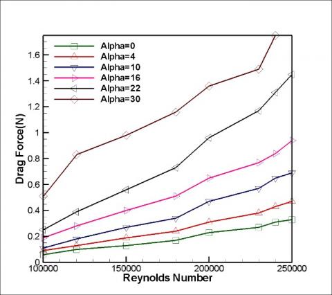
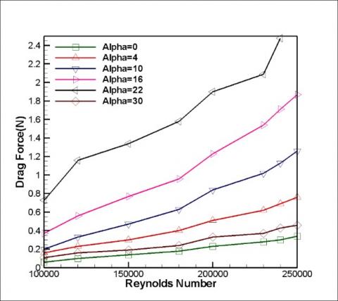
Experiments are done in a wind tunnel on icy and non-icy airfoils and the Reynolds number and drag force are obtained from experimental data and by using equations 1 to 5. So, drag reduction percent are calculated. These tests are done for different attack angles from to . Results for different attack angles are shown in figures 5 and 6 for icy and non-icy airfoils. Drag force increases when Reynolds number rises. Also drag force increases while attack angle grows.
Figure 5. Drag force versus Reynolds number in different attack angles in icy airfoil
Figure 6. Drag force versus Reynolds number in different attack angles in non-icy airfoil
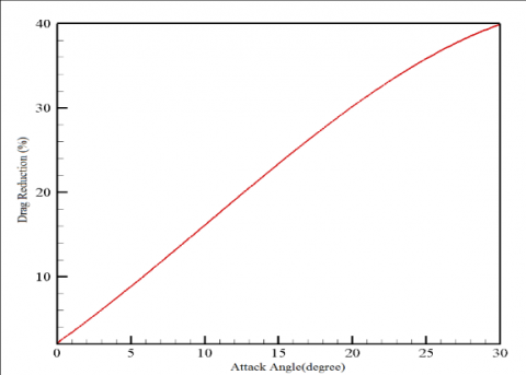
Also, the average drag reduction versus the attack angle has been displayed in Figure 7
Figure 7. Average drag reduction (icy airfoil in comparison with non-icy airfoil) versus attack angle
Results show that the drag reduction is changed from 2 % to 40 % when attack angle is changed from 00 to 300. Due to more roughness of icy airfoil, the friction drag is more for icy airfoil. Roughness of icy airfoil converts laminar flow to turbulent flow. Then due to sharp gradient of velocity near the wall, in the turbulent flow, shear stress on icy airfoil is more than non-icy airfoil. Boundary layer separation is delayed because of turbulent flow. So boundary layer separation happens later in icy airfoil. This event has two effects. First one is increase in the shear stress and second one is decrease in the pressure drag force. Boundary layer separation causes a high pressure part before separation point and a low pressure part after that. As a result, force on the front part of airfoil is more than the back part of airfoil and this effect produces asymmetric pressure distribution or a strong pressure drag force. According to mentioned reasons, pressure drag force on icy airfoil is less than non-icy airfoil. At low attack angles, friction drag and pressure drag are important but at high attack angles, large part of drag force is the pressure drag force. So low pressure drag leads to a low pressure drag force.
Given that pressure drag is less for icy airfoil, total drag force is less, too, especially in a high attack angle. Formation of secondary boundary layer in the icy airfoil is another reason for the drag force reduction. This boundary layer is created under the main boundary layer because of sublimation of ice.
In this paper, an icy airfoil has been conveyed and its drag force has been compared with that of a non-icy airfoil. This study has done in a subsonic wind tunnel experimentally. Results have showed that drag force of icy airfoil is less than non-icy one. This reduction which is function of attack angle, increases when attack angle rises. This reduction is from 2 % to 40 %. The main reason for this reduction is that in icy airfoil, the boundary layer separation happens later than non-icy airfoil. Roughness of airfoil converts laminar flow to turbulent flow then boundary layer separation delayed. The other reason is secondary boundary layer. In this flow, ice converts its shape into vapor and then this vapor makes secondary boundary layer under the primary one.
[1] Zhou B, Wang X, Guo W, Zheng J, Tan SK. (2015). Experimental measurements of the drag force and the near-wake flow patterns of a longitudinally grooved cylinder. Journal of Wind Engineering and Industrial Aerodynamics 145: 30-41. https://doi.org/10.1016/j.jweia.2015.05.013
[2] Gylys J, Paukštaitis L, Skvorčinskienė R. (2012). Numerical investigation of the drag force reduction induced by the two-phase flow generating on the solid body surface. International Journal of Heat and Mass Transfer 55: 7645-7650. https://doi.org/10.1016/j.ijheatmasstransfer.2012.07.078
[3] Abrebekooh YN, Rad M. (2011). Experimental and numerical investigation of drag force over tubular frustum. Scientia Iranica 18: 1133-1137. https://doi.org/10.1016/j.scient.2011.08.027
[4] Khaled M, El-Hage H, Harambat F, Peerhossaini H. (2012). Some innovative concepts for car drag reduction: A parametric analysis of aerodynamic forces on a simplified body. Journal of Wind Engineering and Industrial Aerodynamics 107-108: 36-47. https://doi.org/10.1016/j.jweia.2012.03.019
[5] Nakamura H, Igarashi T. (2008). Omnidirectional reductions in drag and fluctuating forces for a circular cylinder by attaching rings. Journal of Wind Engineering and Industrial Aerodynamics 96: 887-899. https://doi.org/10.1016/j.jweia.2007.06.016
[6] Polidori G, Taïar R, Fohanno S, Mai TH, Lodini A. (2006). Skin-friction drag analysis from the forced convection modeling in simplified underwater swimming. Journal of Biomechanics 39: 2535-2541. https://doi.org/10.1016/j.jbiomech.2005.07.013
[7] Mirzaei M, Ardekani MA, Doosttalab M. (2009). Numerical and experimental study of flow field characteristics of an iced airfoil. Aerospace Science and Technology 13: 267-267. https://doi.org/10.1016/j.ast.2009.05.002
[8] Koomullil RP, Thompson DS, Soni BK. (2003). Iced airfoil simulation using generalized grids. Applied Numerical Mathematics 46: 319-330. https://doi.org/10.1016/S0168-9274(03)00044-8
[9] Tsao JC, Rothmayer AP. (2002). Application of triple-deck theory to the prediction of glaze ice roughness formation on an airfoil leading edge. Computers & Fluids 31: 977-1014. https://doi.org/10.1016/S0045-7930(01)00050-0
[10] Kornilov VI. (2006). Direct measurements of the drag of a body of revolution in an incompressible flow under the action of eddy breakup devices. Thermophysics and Aeromechanics 13: 499-506. https://doi.org/10.1134/S0869864306040032
[11] Kornilov VI. (2010). Effect of vertical large eddy breakup devices on the drag of a flat plate. Thermophysics and Aeromechanics 17: 249-258. https://doi.org/10.1134/S0869864310020101
[12] Leontiev AI, Milman OO. (2014). Hydraulic drag at the condensing steam flow in tubes. Thermophysics and Aeromechanics 21: 755-758. https://doi.org/10.1134/S0869864314060109
[13] Semenov BN. (2009). Strategy of a choice of single-layer compliant coatings for turbulent drag reduction. Thermophysics and Aeromechanics 16: 219-228. https://doi.org/10.1134/S0869864309020061
[14] Rabani M, Faghih AK, Rabani R. (2016). Aerodynamic characteristics investigation of a passenger train under crosswind. Iranian Journal of Science and Technology, Transactions of Mechanical Engineering 40: 139-149. https://doi.org/10.1177%2F0954409718770345
[15] Majumder S, Roy D, Bhattacharjee S, Debnath R. (2014). Experimental investigation of the turbulent fluid flow through a rectangular diffuser using two equal baffles. Journal of The Institution of Engineers (India): Series C 95: 19-29. https://doi.org/10.1007/s40032-014-0100-x
[16] Fouad MA, Zewail TM, Amine NKA. (2017). Effect of drag reducing polymer and suspended solid on the rate of diffusion controlled corrosion in 90° copper elbow. Journal of The Institution of Engineers (India): Series C 98: 261-266. https://doi.org/10.1007/s40032-016-0286-1
[17] Natarajan G, Sahoo N, Kulkarni V. (2015). Optimal forebody shape for minimum drag in supersonic flow. Journal of The Institution of Engineers (India): Series C 96: 5-11. https://doi.org/10.1007/s40032-014-0134-0