OPEN ACCESS
In view of the difficulty in manual monitoring of the operation state of grid servers, this paper develops an operation state prediction method for severs in smart grid based on several innovative techniques. The prediction method consists of two main steps. Firstly, the warning threshold was determined by Chebyshev inequality and improved Rayleigh distribution, and then the upper bound of warning, the value of parameter ε, as well as the abnormal probability of each timepoint were calculated according to the definition of small probability event. Secondly, the back propagation neural network (BPNN) was introduced for time sequence prediction and overall analysis of the previous results, thereby obtaining the future data of CPU utilization of grid servers. The proposed method was proved valid through several experiments. The warning threshold set by our method can warn about abnormalities without sacrificing the scientific operation of the grid, and evaluate the abnormal probability of each data point. The research findings shed new light on the early warning of abnormal server states in smart grids.
data monitoring, chebyshev inequality, rayleigh distribution, back propagation neural network (BPNN)
In the pursuit of sustainable development, many countries are competing to develop the next generation grid that can save energy, reduce emission and produce green power. Taking China for example, much efforts have been paid to design a smart grid, which is independent from and more efficient than traditional grids (Chen et al., 2018). The design process takes into account the latest development of green energy (Tan, 2017).
Big data is ubiquitous in the smart grid system, especially in the monitoring center. In most Chinese grid companies, there is a huge amount of data in the monitoring center, making it difficult to monitor the operation status of grid servers. Once a sever fails, it often takes a long time to identify the failure, not to mention coming up with a timely solution.
Against this backdrop, it is very meaningful to maximize the monitoring efficiency of grid servers by the cutting-edge automation technologies (Wang et al., 2007). An effective monitoring system should be able to analyze the grid data and determine the part of server affected by the failure, allowing operators to solve the problem in a short time (Liu, 2015).
The existing monitoring systems for grid servers mainly focus on the adjustment of CPU, memory and hard drive. For instance, a resource control system (Padala et al., 2009) was designed for containing online model estimator in light of cybernetics and multi-input and multi-output (MIMO) resource controller; this control system captures the complex relationship between application performance and the amount of resource allocation, and supports the automatic adaptation to the dynamically changing application load and demand-driven adjustment of the allocation amount. A dynamic adjustment method (Menasce et al., 2006) was proposed for computing resource allocation according to CPU priority, which varies with the workloads of the virtual machine; considering the migration cost, this approach (Hu et al., 2006) selects the virtual machine to be migrated by weighing CPU utilization and memory size, and predicts the load trend of the server based on the load threshold, aiming to avoid the migration triggered by instantaneous peak loads.
Early warning to the server is essential to the monitoring of the operation state of each device and the elimination of hidden hazard of the smart grid. The related research relies on the prediction of CPU utilization of the server. For example, Reference (Wen et al., 2014) combines the auto regressive integrated moving average (ARIMA) and back propagation neural network (BPNN) into a prediction model for the CPU utilization of the server, such that the server can make timely and accurate response to the change of the application load. Specifically, a server time sequence prediction model was constructed, integrating the advantage of the ARIMA in linear space and that of the BPNN in nonlinear space. Meanwhile, the data structure of server CPU utilization time sequence was divided into the linear part and the nonlinear residual. Next, the general trend of the sequence was predicted by the ARIMA and the nonlinear residual was estimated by the BPNN. The results were combined into a desirable prediction outcome.
In light of the above, this paper puts forward a method to determine adaptive dynamic thresholds based on the improved Chebyshev inequality for Rayleigh distributions, which can effectively predict the server CPU utilization and thus the operation state of smart grid servers. By this method, the data distribution of CPU utilization was analyzed skillfully in light of the probability density of Rayleigh distribution function. Firstly, the CPU utilization values were set according to the definition of small probability event, and the probability of each data point was calculated. Next, the CPU utilization value in future was predicted by the BPNN, and compared against the previous threshold to figure out the time of future failure.
The remainder of this paper is organized as follows: Section 2 analyzes the Chebyshev inequality, introduces and improves the Rayleigh distribution, reviews the BPNN, and prepares an implementation plan for our method; Section 3 carries out experiments on our plan and discusses the experimental results; Section 4 wraps up this paper with several conclusions.
2.1. Analysis of the Chebyshev inequality
Chebyshev inequality is an estimation of the probability of event |X-μ|<ε, where X is a random variable with unknown distribution that determines the event probability (Zhang et al., 2013). Let E(X)=μ and D(X)=σ2 be the mathematical expectation and the variance of X, respectively. Then, the following relationships are valid for any positive integer ε:
$P\{\left| X-\mu \right|\ge \varepsilon \}\le \frac{{{\sigma }^{2}}}{{{\varepsilon }^{2}}}$ (1)
$P\left\{ \left| X-\mu \right|\le \varepsilon \right\}\ge 1-\frac{{{\sigma }^{2}}}{{{\varepsilon }^{2}}}$ (2)
where X is a random variable; ε is a positive integer. The actual meaning of ε is the standard for threshold setting.
Inspired by the Chebyshev inequality, the CPU utilization was introduced to detect the operation abnormality in grid sever at a certain time. Although the probability density is unknown, the mean and variance of CPU utilization in a time period help to judge whether a time point is suspicious. If the value of ε is small, then the grid server is operating normally at the time point. The value of ε has a positive correlation with the difference between the current CPU utilization and the mean CPU utilization. According to Chebyshev inequality, this difference falls between 1-σ2/ε2 and ε. The higher the lower bound, the more likely for the server to operate normally at the corresponding time point. The above method is used to determine the abnormal data points in this paper. Any point above the dynamic threshold was considered as abnormal.
2.2. Rayleigh distribution and improvement
For a random 2D vector, if its two components are independently and normally distributed with equal variance and the mean of zero, then the modulus of this vector must obey the Rayleigh distribution (Liu, 2016). The probability density of Rayleigh distribution can be expressed as:
$f(x)=\frac{x}{{{\sigma }^{2}}}{{e}^{-\frac{{{x}^{2}}}{2{{\sigma }^{2}}}}},x>0$ (3)
where x is the CPU utilization; σ2 is the variance. Data collation reveals that the CPU utilization data mainly fell between 0 and 5, but this pattern weakened with the growth in CPU utilization. To put it more intuitively, the CPU utilization data of host 414# from August 18th to September 18th in 2017 are presented in Figure 1 below.
Figure 1. Distribution of CPU utilization of host 414#
For grid servers, the probability of Rayleigh distribution must decrease monotonously with the growth in the CPU utilization value. Since the CPU utilization data mostly fell between 0 and 5, it is not desirable to implement the Rayleigh distribution formula directly. Thus, this formula was modified according to the actual data.
Taking the derivative of f(x), the probability density of Rayleigh distribution can be converted into:
${f}'(x)=\left( \frac{1}{{{\sigma }^{2}}}-\frac{{{x}^{2}}}{{{\sigma }^{4}}} \right)\times {{e}^{-\frac{{{x}^{2}}}{2{{\sigma }^{2}}}}},x>0$ (4)
If the derivative is 0, x equals 0. In other words, f(x) reaches the maximum value when x is equal to σ. This obviously goes against the face. If equation (4) is rewritten as
${f}'(x)=\left( \frac{1}{{{\sigma }^{2}}}-\frac{k{{x}^{2}}}{{{\sigma }^{4}}} \right)\times {{e}^{-\frac{{{x}^{2}}}{2{{\sigma }^{2}}}}},x>0$ (5)
Then, the peak value of f(x) can be adjusted by controlling the k value according to the actual situation. In this way, the derivative of the new f(x) is always in line with the fact, and the result of integration the new f(x) over 0~+∞ equals 1. Substituting y=ax into equation (5) and integrating the equation over 0~+∞, we have:
$\int_{0}^{+\infty }{\frac{{{a}^{2}}y}{{{\sigma }^{2}}}{{e}^{-\frac{{{a}^{2}}{{y}^{2}}}{2{{\sigma }^{2}}}}}dy},y>0$ (6)
Equation (6) can be rewritten as:
$f(x)=\frac{Ax}{{{\sigma }^{2}}}{{e}^{-\frac{A{{x}^{2}}}{2{{\sigma }^{2}}}}},x>0$ (7)
where A is the adaptive coefficient. If x is equal to μ, then the value of f(μ) reaches the maximum. In this case, the value of A can be determined.
2.3. BPNN
The learning of the BPNN consists of two processes, namely, the forward propagation of the inputs and the backward propagation of the errors. In the forward propagation, the inputs move from the input layer to the output layer via the hidden layer. If the outputs of the output layer differ from the expected outputs, then the output error will be calculated and transmitted back reversely. Then, the weight between the neurons of each layer will be modified to minimize the error (Constantin et al., 2016).
Neurons are the building blocks of the BPNN (Ren, 2015), whose structure is shown in Figure 2. In this figure, the inputs of the BPNN are denoted as xi (i=1,2, …, R), the connection weight between the neurons as ωi (i=1,2, …, R), the threshold (bias value) as b=ωi, and the transfer function as f. Then, the outputs of the BPNN can be expressed as:
$y=f(\sum\nolimits_{i=1}^{R}{{{x}_{i}}{{\omega }_{i}}+b})$ (8)
Let X= (x1, x2, …, xR), W= (ω1,ω2, …, ωR)T and XW+b=n. Then, we have y=f(n).
Figure 2. BPNN structure
In our case, the feedforward network becomes a nonlinear function. Let {Xn} be a time sequence. Then, the CPU utilization can be predicted as:
${{X}_{n+k}}=f({{X}_{n}},{{X}_{n-1}},{{X}_{n-2}},\cdots {{X}_{1}})$ (9)
where f is the analog function; n=1, 2,..., N are the time points; Xn is the CPU utilization at a time point (Zhu et al., 2010). The BPNN prediction can be implemented through the following steps.
2.3.1. Sample extraction and training set construction
Accurate samples are the key to the validity of the established training data set. A rational sampling method should cover all data points according to the features of the time sequence, and select a proper number of samples. Too many samples will cause overfitting and an increase of network complexity; otherwise, a high fitting error will occur in training and hinder network extension.
2.3.2. Dataset pre-processing
In the network, the artificial neuron is described as the processing elements, as they have weighted inputs, transfer functions, and an output. The input of these neurons should be weighted and summarized, forming an activation function (Harikeshava et al., 2017). BPNN has a strict requirement on the input data. Uniform the inputs, the more stable the prediction performance. The data with obvious amplitude variation are not suitable for network inputs.
2.3.3. Design of network structure
To design a sound network structure, the following factors should be determined properly in turns: the number of network layers, the number of output layer nodes, the number of hidden layer nodes, the number of input layer nodes, the activation function in the hidden layer, the training function, the learning function and the activation function in the output layer.
2.3.4. Initialization
The above factors should be initialized and the threshold and connection weights should be determined randomly.
2.3.5. Data input
The sample data should be inputted to the hidden layer and the output layer.
2.3.6. Recalculation
The connection weights and thresholds should be recalculated according to the feedback values.
2.3.7. Termination judgement
If proper inputs are obtained through the recalculation, please return to Step (5). If the error of the output layer is below the pre-set value, the training process should be terminated.
2.3.8. Prediction
The training model can now be used to predict the future trend.
2.4. Our implementation plan
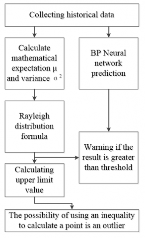
Our implementation plan for predicting the operation state of grid servers covers the following steps: setting up a rational threshold model, verifying the abnormal probability of each data point, predicting the CPU utilization by the BPNN, comparing the predicted value with the threshold, and issuing a warning about the abnormal points. The block diagram for the implementation plan is shown in Figure 3 below.
As shown in Figure 3, the implementation plan contains the following six steps.
Figure 3. The block diagram for the implementation plan
(1) The entire system collected the historical data on CPU utilization.
(2) The probability distribution of CPU utilization data was calculated by the improved Rayleigh distribution function. The variance of CPU utilization data in one month was computed and then the expression of the Rayleigh distribution was obtained. The variance is an adaptive threshold.
(3) The data were updated on a daily basis. In every update, the data of the first day of the current month were discarded, and those of the current day were included. Then, the variance was computed again to obtain the new Rayleigh distribution expression.
(4) The threshold was calculated according to the definition of small probability event.
(5) The threshold was substituted into Chebyshev inequality to calculate the abnormal probability of a data point.
(6) The future CPU utilization was predicted by the BPNN according to the historical data and compared against the previous threshold to determine the time point of failure.
Two threshold setting plans were put forward for the operation state prediction of grid servers. In the first plan, the threshold is determined by Chebyshev inequality and the warning indices obtained from experimental adjustment; in the second plan, the threshold is determined through Chebyshev inequality and improved Rayleigh distribution function according to the definition of small probability event.
According to the first plan, the probability of event |X-μ|<ε was estimated by Chebyshev inequality. The probability estimates of Chebyshev inequality are listed in Table 1 below.
Table 1. Statistical table of probability estimates
|
ε |
σ2/ε2 |
1-σ2/ε2 |
|
$\sqrt { 3 / 2 \sigma }$ |
2/3 |
1/3 |
|
$\sqrt {2 \sigma }$ |
1/2 |
1/2 |
|
$\sqrt { 5 / 2 \sigma }$ |
2/5 |
3/5 |
|
$\sqrt { 3 \sigma }$ |
1/3 |
2/3 |
|
$\sqrt { 7 / 2 \sigma }$ |
2/7 |
5/7 |
|
$ 2 \sigma $ |
1/4 |
3/4 |
The values of the adjustment coefficients ξ1 and ξ2 must be set manually before determining the value of ε. Here, these two coefficients and the thresholds T1 and T2 are defined as:
$\begin{align} & \left\{ \begin{matrix} {{T}_{1}}=\frac{(1-\frac{{{\sigma }_{k}}^{2}}{{{\varepsilon }_{1}}^{2}})+0.5}{2},{{\varepsilon }_{1}}=\sqrt{2}\sigma +{{\xi }_{1}}\sigma \\ {{T}_{2}}=\frac{(1-\frac{{{\sigma }_{k}}^{2}}{{{\varepsilon }_{2}}^{2}})+0.5}{2},{{\varepsilon }_{2}}=\sqrt{2}\sigma -{{\xi }_{2}}\sigma \\\end{matrix} \right. \\ & (0<{{\xi }_{1}},{{\xi }_{2}}<1) \\\end{align}$ (10)
To classify CPU utilization data points, the segmented function M can be customized as:
$M=\left\{ \begin{matrix} 1,(1-\frac{{{\sigma }^{2}}}{{{\varepsilon }^{2}}})\ge {{T}_{1}} \\ 0,(1-\frac{{{\sigma }^{2}}}{{{\varepsilon }^{2}}})\le {{T}_{2}} \\\end{matrix},\varepsilon =\sqrt{2}\sigma \right.$ (11)
If M=1, then the current CPU utilization is abnormal; if M=0, then the current CPU utilization is normal; if T2<1-σ2/ε2<T1, then the current time point is suspicious. Different values of ξ1 and ξ2 (0<ξ1, ξ2<1) were selected to differentiate between normal points, abnormal points and suspicious points, and determine the values of T1 and T2. The values of T1 and T2 can be derived from ξ1 and ξ2 through the following adaptive threshold setting rules:
(1) If ξ1=ξ2=0.5, then T1=2.0821 and T2=0.6678;
(2) If ξ1=0.6 and ξ2=0.4, then T1=-2.0821 and T2=0.8578.
The results of this plan show that the CPU utilization was abnormal at most time points, which is obviously untrue. Some normal data must have been wrongly judged as suspicious. For example, misjudgment many occur if a host is suddenly visited, leading to an increase in CPU utilization. In addition, this plan is too subjective to reflect the objective situation.
According to the second plan, the threshold was determined by the Chebyshev inequality and the improved Rayleigh distribution function according to the definition of small probability events. Considering the huge amount of data and the heavy presence of invalid data in our case, host 414# and host 507# were randomly selected after data filtering for further analysis.
(1) For host 414#, the mathematical expectation, standard deviation and variance were computed as μ=1.4154, σ=1.068 and σ2=1.03362, respectively. Then, the A=0.5331 was obtained by equation (10). The processing results of this host are presented in Table 2.
Table 2. Processing results of host 414#
|
|
statistic |
|
|
mean |
standard deviation |
variance |
|
1.415 |
1.033 |
1.068 |
Next, the threshold can be obtained by formula (7) as $P \left( X _ { 0 } > x > 0 \right) = \int _ { 0 } ^ { x _ { 0 } } f ( x ) d x = 0.99$. After that, the value of X0 can be determined as 4.300 on the Matlab.
(2) For host 507#, the mathematical expectation, standard deviation and variance were computed as μ=1.3129, σ=0.6260 and σ2=0.392, respectively. Then, the A=0.5331 was obtained by equation (10). The processing results of this host are presented in Table 3.
Table 3. Processing results of host 507#
|
|
statistic |
|
|
mean |
standard deviation |
variance |
|
1.312 |
0.626 |
0.392 |
According to equation (10), this is a probability density function. The definite integral of equation (10) is consistent with that of Step (1), and the value of X0 was determined as 3.988.
The above operations show that the improved Rayleigh distribution model can approximate the actual distribution of CPU utilization. The adaptive threshold was calculated scientifically according to the definition of small probability event. By this method, it is learned that the threshold for host 414# on September 19th was 4.300. In other words, the system will issue a warning when the CPU utilization exceeds 4.300. For host 507#, the warning will be released when the CPU utilization surpasses 3.988.
Next, the reliability of the upper bound obtained by Rayleigh distribution was verified by Chebyshev inequality. According to the formula $P \{ | X - \mu | < \varepsilon \} \geq 1 - \frac { \sigma ^ { 2 } } { \varepsilon ^ { 2 } }$ the value of ε was obtained from ε-μ=X0, and then the abnormal probability of each point was calculated.
(1) For host 414#, the value of ε can be determined as 5.7154 from ε-μ=X0. In this case, at least 96.73% of the data points in the warning were probably abnormal.
(2) For host 507#, the value of ε can be determined as 5.3009 from ε-μ=X0. In this case, at least 98.60% of the data points in the warning were probably abnormal.
The experimental data demonstrate the reliability of the predicted results. The predicted points can be basically viewed as abnormal. Hence, this plan can output an adaptive threshold for the operation state prediction of grid servers.
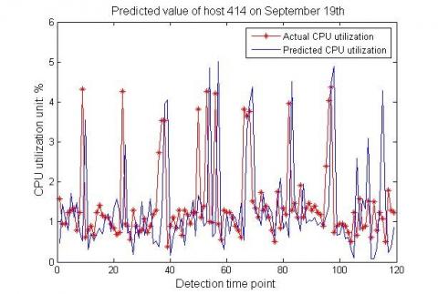
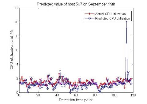
After the threshold was determined, the next step is to predict the CPU utilization, and thus identify the operation state of grid servers and identify potential risks. Based on the historical data, the CPU utilization was predicted by the BPNN. Specifically, the CPU utilization of the sixth day was forecasted based on those of the previous five days, and contrasted against the measured data. Then, the data of the last five time points were relied on to predict those of the next time point. After that, the predicted data were combined with the data of the last four time points to further predict the new next time point. These processes were repeated until all time points had been predicted. Then, the CPU utilization of each host was calculated and compared with the predicted data (Figures 4 and 5).
Figure 4. Comparison between measured and predicted CPU utilizations of host 414# on September 19th
Figure 5. Comparison between measured and predicted CPU utilizations of host 507# on September 19th
The comparisons verify the accuracy of this prediction method. Next, the above method was adopted to predict the CPU utilization at the next 15 time points. The predicted results were contrasted against the threshold to find the potential abnormal points.
(1) For host 414#, the CPU utilizations for the next 15 time points were predicted as: 0.15212, 0.45288, 0.62012, 29.340, 1.2280, 0.83339, 10.370, 13.546, 13.204, 13.599, 1.1811, 0.76360, 0.83339, 0.83339 and 0.15186. As the threshold was 4.300, the abnormal values include 29.340, 10.370, 13.546, 13.204 and 13.599.
(2) For host 507#, the CPU utilizations for the next 15 time points were predicted as: 0.29169, 0.4356, 2.4965, 2.6374, 0.21653, 2.9053, 1.4561, 1.7324, 5.0202, 2.8766, 6.5453, 0.30237, 0.94157, 5.0142 and 5.1322. As the threshold was 3.988, the abnormal values include 6.5453, 5.0142 and 5.1322.
Compared with the data distributions in Figures 5 and 6, the above predicted data were much greater than those at normal time points. The result indicates that the threshold setting is rational. In the future, the warning system will react in advance and locate the abnormalities as long as the CPU utilization trend goes in line with the predicted trend.
The traditional Chebyshev inequality faces a high computing cost, a limited application range, and high subjectivity in dealing with adaptive dynamic threshold. In this paper, the adaptive threshold is determined by the Rayleigh distribution function, which has been improved according to the actual situation, before the Chebyshev inequality is introduced to determine the abnormal probability of time points.
Coupled with the adaptive threshold, the BPNN was adopted to predict the CPU utilization of grid servers in the next 15 time points according to the historical data. This arrangement makes full use of the BPNN’s strength in predicting time sequences and solving nonlinear complex data problems. In this way, the author successfully predicted the CPU utilization of grid servers in future and realized pre-warning of server abnormalities.
Chen J. D., Sheng G. H., Wu J. J. (2018). Application status and prospect of big data technology in smart grid. High Voltage Apparatus, Vol. 54, No. 1, pp. 35-43. http://www.cnki.com.cn/Article/CJFDTotal-GYDQ201801006.htm
Constantin B., Stefan K., Antheia D. (2016). Artificial neural network based monthly load curves forecasting. Applied Computational Intelligence and Informatics (SACI) 2016 IEEE 11th International Symposium, pp. 237-242. https://doi.org/10.1109/SACI.2016.7507378
Harikeshava R., Shyam S. M., Vaira V. (2017). ANN model for predicting the intergranular corrosion susceptibility of friction stir processed aluminium alloy AA5083. Communication and Electronics Systems (ICCES), 2017 2nd International Conference, pp. 716-720. https://doi.org/10.1109/CESYS.2017.8321174
Hu Z. G., Ouyang S., Ge C. K. (2006). Resource load balancing method for decreasing energy consumption under cloud environment. Journal of Computer Engineering, Vol. 38, No. 5, pp. 53-55. http://dx.doi.org/10.3969/j.issn.1000-3428.2012.05.014
Liu H. (2015). Research on data center adaptive energy efficiency optimization system. Shandong University, pp. 23-25. http://cdmd.cnki.com.cn/Article/CDMD-10422-1016031005.htm
Liu Z. F. (2016). Two sequential weighted probability ratio tests based on Rayleigh distribution. East China Normal University. http://cdmd.cnki.com.cn/Article/CDMD-10269-1016141642.htm
Menasce D. A., Bennani M. N. (2006). Autonomic virtualized environments. Autonomicand Autonomous Systems, 2006 International Conference on IEEE, pp. 16-21. https://doi.org/10.1109/ICAS.2006.13
Padala P., Hou K. Y., Shin K. G. (2009). Automated control of multiple virtualized resources. The 4th ACME Uropean Conference on Computer Systems, pp. 13-26. https://doi.org/10.1016/S0014-3057(97)00063-3
Ren S. J. (2015). Research on evaluation methods of real estate along urban rail transit based on BP neural network. Beijing Jiaotong University. http://cdmd.cnki.com.cn/Article/CDMD-10004-1015611238.htm
Tan Y. (2017). Research on grid big data governance system. Journal of Electronic Technology and Software Engineering, Vol. 24, No. 05, pp. 182-183. http://www.cnki.com.cn/Article/CJFDTotal-DZRU201705131.htm
Wang S., Xiao Y. Q., Liu D. W. (2007). Research on key technologies of memory database. Journal of Computer Application, Vol. 27, No. 10, pp. 2353-2357. http://dx.doi.org/10.3969/j.issn.1000-5641.2014.05.010
Wen J. (2014). Research on virtual machine dynamic deployment method based on CPU utilization prediction. Northeastern University, pp. 5-11. http://cdmd.cnki.com.cn/Article/CDMD-10145-1016020591.htm
Zhang K., Wang C., Wang C. (2013). An adaptive threshold background modeling algorithm based on Chebyshev's inequality. Journal of Computer Science, Vol. 40, No. 4, pp. 287-297. http://dx.doi.org/10.3969/j.issn.1002-137X.2013.04.062
Zhu K., Wang Z. L. (2010). Proficient in MATLAB neural network. Beijing: Publishing House of Electronics Industry, pp. 104. http://xueshu.baidu.com/usercenter/paper/show?paperid=f81dc481c852ac569773e29aee9b79af