OPEN ACCESS
In view of the importance of fast and accurate forward modelling in electrical numerical simulation, this paper derives the finite-element equation for 2D geoelectrical field with a point current source, and introduces the theoretical formulas under different boundary conditions (i.e. Dirichlet and mixed boundary conditions). On this basis, forward simulations were carried out at the electrical contrasts of 1:10 and 1:100 between a low resistance body in uniform medium and the background field, aiming to compare the simulation results of the body under the two boundary conditions. The comparison shows that the position and range of the low resistance body were well simulated under the mixed boundary condition; however, when the electrical contrast increased to 1:100, the position and range of the low resistance body simulated under the Dirichlet boundary condition deviated greatly from the actual results. Owing to the incomplete projection, an artefact appeared below the anomalous body. The artifact, lighter than the anomalous body, has much less impact on the positioning of the anomalous body than on the range judgement. By contrast, the position of the low-resistance body was imaged relatively accurately under the mixed boundary condition, and the range of the image body was similar to the size of the low-resistance body in the model. Considering the good imaging effects at high and low electrical contrasts and the variety of application scenarios, the finite-element simulation under the mixed boundary condition can be promoted to solve 2.5D and 3D problems.
resistivity tomography (RT), dirichlet boundary condition, mixed boundary condition, 2D geoelectric field with a point power source
Resistivity tomography (RT) has been applied successfully since the early 1980s. Compared with conventional resistivity exploration methods, the RT enjoys a low cost and high efficiency in the exploration of roadbed, minerals and hydrogeology, and provides an ideal solution to many real-world problems.
In 1987, Shima and Sakayama coined the term RT and put forward an inverse interpretation method. Since then, the RT has been investigated both theoretically and practically from multiple angles. Relying on finite-difference method, Dey et al. realized the forward numerical simulation of the resistivity of 3D models in any shape, examined the surface response of low-resistance anomalous body of simple rule block model under dipole-dipole device, and simulated the anomalous surface response of low-resistance body when the current source is at a certain depth of the well. Mizunaga et al. used the finite difference method to complete forward numerical simulation of the hole-surface resistivity method under t point current source and vertical line source, and extended the numerical simulation to the hole-surface resistivity method under the current source of any shape. J.H. Coggon introduced the finite-element method into numerical simulation of electrical exploration. By improving the meshing method, William L. Rodi and Rijo preliminarily increased the computing speed and accuracy of the forward modeling.
Inspired by the previous research into forward numerical simulation (Tabbagh et al., 2000; Kim et al., 2001; Shima & Sakayama, 1987; Sasaki, 1994; Shima, 1990; Binley et al., 2002; Cassiani et al., 2009; Chambers et al., 2004; Daily & Ramirez, 1995; Daily et al., 1992; Deiana et al., 2007; Descloitres et al., 2008; Rocroi et al., 1985; Ramazi et al., 2009; Hattula & Rekola, 2000), this paper re-introduces different boundary conditions by establishing a forward model, compares the forward results of finite-element simulation of RT images acquired under Dirichlet boundary condition and mixed boundary condition, and simulates the response features (geometric features and burial features) at different electrical contrasts between the low-resistance anomalous body and the surrounding rock medium. The research findings lay a solid basis for the selection of proper boundary condition for forward numerical simulation of different geological models (Ushijima et al., 1990; Sill & Ward, 1978; Suparno et al., 2005; Supriyanto et al., 2005).
To disclose the relationship between the new boundary condition and the numerical solution, the remainder of this paper consists of formula derivation, boundary condition, numerical simulation analysis of geoelectric model, and conclusions. The conclusions provide a theoretical basis for the further study of delimited boundary condition.
2.1. Derivation of the finite-element equation of 2D geoelectric field with a point power source
Let A(x0, y0, z0) be the coordinates of the point power source in an infinite medium whose resistivity is ρ(x, y, z), and I be the current intensity of the point power source. In the coordinate system, the x and y axes were arranged along the direction of the geological body while the z axis was vertically downward. Then, the potential function U of stable current field satisfies the following differential equation:
$\nabla \cdot \left( \sigma \cdot \nabla U \right)=-I\delta \left( r-{{r}_{A}} \right)$ (1)
where σ is the dielectric conductivity; δ is the Dirac equation; U is the potential at any point on the surface or in the medium; I is the supply current intensity; r is the field point radius vector; rA is the source point radius vector.
Since
for a 2D geoelectric profile, equation (1) can be rewritten as:$\nabla \cdot \left[ \sigma \left( x,z \right)\nabla U\left( x,y,z \right) \right]=-I\delta \left( x-{{x}_{0}} \right)\delta \left( y-{{y}_{0}} \right)\delta \left( z-{{z}_{0}} \right)$ (2)
Applying Fourier transform to the basic differential equation of the steady current field along the y axis, we have:
$\phi \left( x,k,z \right)=\int_{0}^{\infty }{U\left( x,y,z \right)\cos \left( k\cdot y \right)dy}$ (3)
Transforming the potential U in space (x, y, z) to the generalized potential
of space, we have:$\nabla \cdot \left[ \sigma \left( x,z \right)\nabla \overline{U}\left( x,{{K}_{y}},z \right) \right]-K_{y}^{2}\sigma \left( x,z \right)\overline{U}\left( x,{{K}_{y}},z \right)=-\frac{1}{2}\delta \left( x-{{x}_{0}} \right)\delta \left( z-{{z}_{0}} \right)$ (4)
where Kyis the spatial wavenumber; δ is the Dirac function.
2.2. Delimited boundary condition
(1) Dirichlet boundary condition
The unique solution of equation (4) can be determined only under the definite condition of the boundary. In this paper, the Dirichlet boundary condition is selected, that is, the potential value φ is given on the boundary, because the boundaries must be far away from the field source and the non-uniform body. The Dirichlet boundary condition can be expressed as [21~30]:
$U\left( x,y,z \right)\left| _{\Gamma } \right.=\varphi \left( x,y,z \right)$ (5)
As the value of φ(x, y, z) is difficult to be obtained by formulas, one of the following two conditions is often adopted:
①
The boundary potential is set to zero; ② It is assumed that $\frac{\partial \varphi}{\partial n}=0$ on the boundary.During the y direction Fourier transform of the U in equation (4), the cosine transform was applied with an integration interval between 0 and ∞, for potential U(x, y, z) is symmetric with respect to the plane xz, i.e. U(x, y, z)=U(x, -y, z).
$\widetilde{U}\left( x,k,z \right)=\int_{0}^{\infty }{U\left( x,y,z \right)\cos kydy}$ (6)
Considering the integral property of δ function, the δ function in equation (4) satisfies the following condition:
$\frac{1}{2}\delta \left( A \right)=\frac{1}{2}\delta \left( {{x}_{A}} \right)\delta \left( {{z}_{A}} \right)=\int_{0}^{\infty }{\delta \left( {{x}_{A}} \right)}\delta \left( {{y}_{A}} \right)\delta \left( {{z}_{A}} \right)\cos kydy$ (7)
Substituting equations (6) and (7) into equation (4), we have:
$\frac{\partial }{\partial x}\left( \sigma \frac{\partial \widetilde{U}}{\partial x} \right)+\frac{\partial }{\partial z}\left( \sigma \frac{\partial \widetilde{U}}{\partial z} \right)-{{k}^{2}}\sigma \widetilde{U}=-I\delta \left( A \right)$ (8)
For $\frac{\partial \varphi}{\partial n}=0$ on the boundary, the normal lies in the plane xz and has nothing to do with y. Thus, we have:
$F\left[ {{\left. \frac{\partial U}{\partial n} \right|}_{\Gamma }} \right]={{\left. \frac{\partial \varphi }{\partial n} \right|}_{\Gamma }}=0$ (9)
Equation (5) can be transformed into:
$\widetilde{U}\text{=}F\left[ {{\left. \frac{\partial U}{\partial n} \right|}_{\Gamma }} \right]=\int_{0}^{\infty }{\frac{c}{\sqrt{{{r}^{2}}+{{y}^{2}}}}}\cos kydy=c{{K}_{0}}\left( kr \right)$ (10)
where r falls within the profile passing through point U(0,0,0) and perpendicular to y; Γ∞ boundary is the distance from a point to U(0,0,0); K0 is the zero-order modified Bessel function of the second kind. The differential quotient of K0(x) is:
$\frac{d}{dx}{{K}_{0}}\left( x \right)=-{{K}_{1}}\left( x \right)$ (11)
K1 is the is the first-order modified Bessel function of the second kind. Taking the derivative of equation (10) in the normal n, we have:
$\frac{\partial \widetilde{U}}{\partial n}=\frac{\partial \widetilde{U}}{\partial r}\frac{\partial r}{\partial n}=-ck{{K}_{1}}\left( kr \right)\cos \left( r,n \right)$ (12)
From equations (11) and (12), we have:
$\frac{\partial \widetilde{U}}{\partial n}+{{\left. k\frac{{{K}_{1}}\left( kr \right)}{{{K}_{0}}\left( kr \right)} \right|}_{\Gamma }}=0$ (13)
Then, the generic function can be established as:
$I\left( \widetilde{U} \right)\text{=}\int\limits_{\Omega }{\left[ \frac{\sigma }{2}{{\left( \nabla \widetilde{U} \right)}^{2}}+\frac{1}{2}{{k}^{2}}\sigma {{\widetilde{U}}^{2}}-Ix\left( A \right)\widetilde{U} \right]}d\Omega $ (14)
where the area Ω is surrounded by the surface boundary Γs and the infinity boundary Γ∞. The corresponding variational problem can be expressed as:
$\begin{align} & \delta I\left( \widetilde{U} \right)\text{=}\int\limits_{\Omega }{\left[ \sigma \nabla \widetilde{U}\cdot \nabla \delta \widetilde{U}+{{k}^{2}}\sigma \widetilde{U}\delta \widetilde{U}-I\delta \left( A \right)\delta \widetilde{U} \right]} \\ & =\int\limits_{\Omega }{\nabla \cdot \left( \sigma \widetilde{U}\delta \widetilde{U} \right)d\Omega +\int\limits_{\Omega }{\left[ -\nabla \cdot \left( \sigma \nabla \widetilde{U} \right)+{{k}^{2}}\sigma \widetilde{U}-I\delta \left( A \right) \right]}}\delta \widetilde{U}d\Omega \\\end{align}$ (15)
Substituting equations (9) and (13) into equation (15), we have:
$\begin{align} & F\left( \widetilde{U} \right)\text{=}\int_{\Omega }{\left[ \frac{\sigma }{2}{{\left( \nabla \widetilde{U} \right)}^{2}}+\frac{1}{2}{{k}^{2}}\sigma {{\widetilde{U}}^{2}}-I\delta \left( A \right)\widetilde{U} \right]}d\Omega \\ & +\int_{\Gamma }{\sigma \frac{k{{K}_{1}}\left( kr \right)}{k{{K}_{0}}\left( kr \right)}\cos \left( r,n \right){{\widetilde{U}}^{2}}d\Gamma } \\\end{align}$ (16)
The $\tilde{U}$ of the split node can be obtained by solving the variational problem of equation (16) through finite-element method. The $\tilde{U}$ corresponds to a specific wave number k. The potential U can be obtained via inverse Fourier transform of a group of $\tilde{U}$ values corresponding to different k values.
(2) Mixed boundary condition
Mixed boundary condition can be expressed as:
${{\left. \left( \frac{\partial U}{\partial n}+AU \right) \right|}_{\Gamma }}=\varphi \left( x,y,z \right)$ (17)
where A is a known positive number.
Therefore, the boundary condition of equation (4) can be transformed into the following boundary value problem [31~36]:
$\left. \begin{matrix} \frac{\partial }{\partial x}\left( \sigma \frac{\partial \overline{U}}{\partial x} \right)+\frac{\partial }{\partial z}\left( \sigma \frac{\partial \overline{U}}{\partial z} \right)-{{\lambda }^{2}}\sigma \overline{U}={{f}_{1}} \\ {{\left. \frac{\partial \overline{U}}{\partial n} \right|}_{{{\Gamma }_{1}}}}=0 \\ {{\left. \left( \frac{\partial \overline{U}}{\partial n}+A\overline{U} \right) \right|}_{{{\Gamma }_{2}}}}=0 \\\end{matrix} \right\}$ (18)
where
${{f}_{1}}=-\frac{1}{2}\sum\limits_{k-1}^{n}{{{I}_{k}}\delta \left( x-{{x}_{k}},z-{{z}_{k}} \right)}$ (19)
$A\text{=}\lambda \frac{{{k}_{1}}\left( \lambda r \right)}{{{k}_{0}}\left( \lambda r \right)}\cos \theta \left( r\ne y \right)$ (20)
where Γ1 is the ground boundary; Γ2 is the remaining boundary; Ik is the current intensity of the k-th point current source; k1(λr) is the first-order modified Bessel function; k0(λr) is the zero-order modified Bessel function; θ is the angle between the radius vector r from the power point to the boundary point and the outer normal n of boundary.
Since the A in equation (20) is a constant, the following can be obtained through the Fourier transform of the U in equation (17):
$\varphi \left( x,y,z \right)=A{{k}_{0}}\left( \lambda r \right)$ (21)
where k0(λr) is the zero-order modified Bessel function, and
$\frac{\partial \varphi }{\partial n}=-A\lambda {{k}_{1}}\left( \lambda r \right)\cos \theta $ (22)
where k1(λr) is the first-order modified Bessel function; θ is the angle between the radius vector r and the outer normal n.
According to equation (21), we have:
$A\text{=}\frac{\varphi \left( x,y,z \right)}{{{k}_{0}}\left( \lambda r \right)}$ (23)
Substituting equation (23) into equation (22), we have:
$\frac{\partial \varphi }{\partial n}+\lambda \frac{k{}_{1}\left( \lambda \cdot r \right)}{{{k}_{0}}\left( \lambda \cdot r \right)}\varphi \cos \theta =0$ or $\frac{\partial \varphi }{\partial n}+\alpha \varphi \cos \theta =0$ (24)
Substituting the mixed boundary condition (24) after the variation of equation (17) into the condition, equation (18) can be converted into an equivalent variational problem [37~42]:
\[W\left( \overline{U} \right)=\iint\limits_{D}{\left\{ \begin{align} & \sigma \left[ {{\left( \frac{\partial \overline{U}}{\partial x} \right)}^{2}}+{{\left( \frac{\partial \overline{U}}{\partial z} \right)}^{2}} \right]+ \\ & \sigma K_{y}^{2}{{\overline{U}}^{2}}-I\delta \left( x-{{x}_{0}} \right)\delta \left( z-{{z}_{0}} \right)\overline{U} \\\end{align} \right\}dxdz+\frac{1}{2}\int\limits_{T}{\sigma a\overline{U}ds}}\] (25)
where I is the current intensity; Γ is the boundary of D, the area of the 2D geoelectric profile; ds is the integral variable of the integrals along the boundary, that is:
$a={{k}_{y}}\frac{{{k}_{1}}\left( {{k}_{y}}r \right)}{{{k}_{0}}\left( {{k}_{y}}r \right)}\cos \theta $ (26)
where k0 and k1 are zero-order and first-order modified Bessel functions, respectively; θ is the angle between the radius vector r from the power point to the boundary point and the outer normal n of boundary. Then, the real potential U can be obtained through the following steps: discretizing the target area; solving the generalized potential $\bar{U}$ by the finite-element method; applying inverse Fourier transform to the generalized potential $\bar{U}$.
(1) Numerical simulation and analysis at the electrical contrast of 1:10 between the anomalous body and the background field
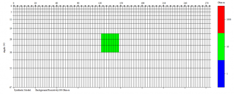
As shown in Figure 1(a), the dipole sounding observation system is adopted in the test model. The parameters were configured as follows: the electrode spacing is 5m, the model thickness is 67m, the surrounding rock resistivity is 100Ω·m, the anomalous body ρ1 (green) resistivity is 10Ω·m, and the electrical contrast is 1:10. The model was used to simulate low-resistance columnar anomalies in a uniform space. The forward model and coordinate system are presented in Figure 1(a).
(a) Forward model at the electrical contrast of 1:10 (between the low resistance anomalous body and the background field in a uniform space)
(b) Image of anomalous body obtained by forward simulation under Dirichlet boundary condition
(c) Image of anomalous body obtained by forward simulation under mixed boundary condition
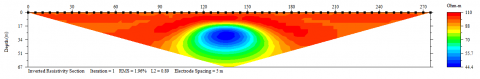
(d) Image of anomalous body obtained by least squares inverse simulation
Figure 1. The test model
As shown in Figures 1(b) and 1(c), the imaging position and range of the anomalous body differed greatly with the selected boundary condition. The image of the low-resistance body fluctuated greatly under the Dirichlet boundary condition. Theoretical derivation shows that, after a certain distance, the imaged body is either smaller or larger than the anomalous body in the model. Comparing Figures 1(a) and 1(b), it can be seen that the Dirichlet boundary condition caused a huge deviation of the anomalous body position in the image from that in the model, and the size of the imaged body was smaller than the size of the anomalous body in the model. By contrast, the position of the low-resistance body was imaged relatively accurately under the mixed boundary condition, and the range of the image body was similar to the size of the low-resistance body in the model.
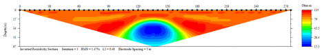
Next, the potential value acquired by the forward calculation under the mixed boundary condition in Figure 1(c) was taken as the prior information, and substituted into the inverse iteration of the model, that is, solving the matrix equation of the least squares method. In this way, the image of anomalous body was acquired by least squares inverse simulation (Figure 1(d)). The iterated image shows that the inverse iteration results closely reflected the position and size of the anomalous body in the model. In the image, the position of the low-resistance body was between 120m and150m in horizontal distance, and between 24m and 38m in depth. The position was basically the same as that in the model. Hence, the RT can reliably image the low resistance body under mixed boundary condition.
(2) Numerical simulation and analysis at the electrical contrast of 1:100 between the anomalous body and the background field
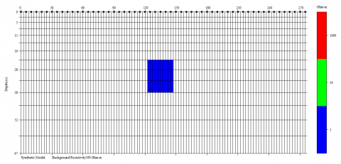
As shown in Figure 2(a), the dipole sounding observation system is adopted in the test model. The parameters were configured as follows: the electrode spacing is 5m, the model thickness is 67m, the surrounding rock resistivity is 100
, the anomalous body (green) resistivity is 10 , and the electrical contrast is 1:100. The model was used to simulate low-resistance columnar anomalies in a uniform space. The forward model and coordinate system are presented in Figure 2(a).(a) Forward model at the electrical contrast of 1:100 (between the low resistance anomalous body and the background field in a uniform space)
(b) Image of anomalous body obtained by forward simulation under Dirichlet boundary condition
(c) Image of anomalous body obtained by forward simulation under mixed boundary condition
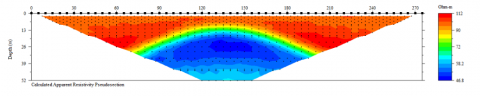
(d) Image of anomalous body obtained by least squares inverse simulation
Figure 2. The test model
As shown in Figures 2(b) and 2(c), when the electrical contrast between the low resistance anomalous body and the background field increased to 1:100 while other conditions remained the same, the imaging position and range of the anomalous body was still accurately simulated under the mixed boundary condition, but image of the low-resistance body fluctuated greatly under the Dirichlet boundary condition. This agrees well with the theoretical derivation that, after a certain distance, the imaged body is either smaller or larger than the anomalous body in the model under the Dirichlet boundary condition. Comparing Figures 1(a) and 1(b), it can be seen that the Dirichlet boundary condition caused a huge deviation of the anomalous body position in the image from that in the model, and the size of the imaged body was larger than the size of the anomalous body in the model. Owing to the incomplete projection, an artefact appeared below the anomalous body. The artifact, lighter than the anomalous body, has much less impact on the positioning of the anomalous body than on the range judgement. By contrast, the position of the low-resistance body was imaged relatively accurately under the mixed boundary condition, and the range of the image body was similar to the size of the low-resistance body in the model.
Next, the potential value acquired by the forward calculation under the mixed boundary condition in Figure 2(c) was taken as the prior information, and substituted into the inverse iteration of the model, that is, solving the matrix equation of the least squares method. In this way, the image of anomalous body was acquired by least squares inverse simulation (Figure 2(d)). The iterated image shows that the inverse iteration results closely reflected the position and size of the anomalous body in the model. In the image, the position of the low-resistance body was between 120m and150m in horizontal distance, and between 24m and 38m in depth. The position was basically the same as that in the model. Hence, the RT can reliably image the low resistance body under mixed boundary condition, despite the nine-fold increase in the electrical contrast, sensitivity and impedance influence.
In this paper, the finite-element method is selected for non-uniform grid simulation of the electrical features at different electrical contrasts between low-resistance anomalous body in a uniform medium and background field. Through forward numerical simulation, it is discovered that the position and range of the low-resistance body were accurately simulated under the mixed boundary condition. Under the Dirichlet boundary condition, however, deviation appeared in the simulated range of the low-resistance body with the growth in the electrical contrast. After a certain distance, the imaged body is either smaller or larger than the anomalous body in the model, and its simulated position deviates from the actual position under the Dirichlet boundary condition.
To sum up, the more the grids in finite-element simulation, the greater the electrical variation of the anomalous body, and the more obvious the difference between the simulated results between the Dirichlet and mixed boundary conditions. Considering the good imaging effects at high and low electrical contrasts under the mixed boundary condition, this research method can be promoted to solve 2.5D and 3D problems. Further studies are needed to develop suitable theoretical and practical methods for 3D geoelectric simulation.
Binley A., Winship P., West L. J., Pokar M., Middleton R. (2002). Seasonal variation of moisture content in unsaturated sandstone inferred from borehole radar and resistivity. Journal of Hydrology, Vol. 267, No. 3–4, pp. 160–172. https://doi.org/10.1016/S0022-1694(02)00147-6
Cassiani G., Godio A., Stocco S., Villa A., Deiana R., Frattini P., Rossi M. (2009). Monitoring the hydrologic behaviour of a mountain slope via time-lapse electrical resistivity tomography. Near Surface Geophysics, Vol. 7, No. 5-6, pp. 475–486. https://doi.org/10.3997/1873-0604.2009013
Chambers J. E., Loke M. H., Ogilvy R. D., Meldrum P. I. (2004). Noninvasive monitoring of DNAPL migration through a saturated porous medium using electrical impedance tomography. Journal of Contaminant Hydrology, Vol. 68, No. 1-2, pp. 1–22. https://doi.org/10.1016/S0169-7722(03)00142-6
Daily W., Ramirez A. (1995). Electrical-resistance tomography during in-situ trichloroethylene remediation at the Savanna River Site. Journal of Applied Geophysics, Vol. 33, No. 4, pp. 239–249. https://doi.org/10.1016/0926-9851(95)90044-6
Daily W., Ramirez A., Labrecque D., Nitao J. (1992). Electrical-resistivity tomography of vadose water-movement. Water Resources Research, Vol. 28, No. 5, pp. 1429–1442. https://doi.org/10.1029/91WR03087
Deiana R., Cassiani G., Kemna A., Villa A., Bruno V., Bagliani A. (2007). An experiment of non-invasive characterization of the vadose zone via water injection and cross-hole time-lapse geophysical monitoring. Near Surface Geophysics, Vol. 5, No. 3, pp. 183–194. https://doi.org/10.3997/1873-0604.2006030
Descloitres M., Ruiz L., Sekhar M., Legchenko A., Braun J. J., Kumar M., Subramanian S. (2008). Characterization of seasonal local recharge using electrical resistivity tomography and magnetic resonance sounding. Hydrological Processes, Vol. 22, No. 3, pp. 384-394. https://doi.org/10.1002/hyp.6608
Hattula A., Rekola T. (2000). Exploration geophysics at the Pyhasalmi mine and grade control work of the Outokumpu Group. Geophysics, Vol. 65, No. 6, pp. 1961-1969. https://doi.org/10.1190/1.1444879
Kim J. S., Han S. H., Ryang W. H. (2001). On the use of statistical methods to interpret electrical resiaivity data from the Eumsung basin (Cretaceous), Korea. Journal of Applied Geophysics, Vol. 48, No. 4, pp. 199-217. https://doi.org/10.1016/S0926-9851(01)00107-0
Ramazi H., Nejad M. R. H., Firoozi A. (2009). Application of integrated geoelectrical methods in Khenadarreh (Arak, Iran) graphite deposit exploration. Journal of the Geological Society of India, Vol. 74, No. 2, pp. 260-266. https://doi.org/10.1007/s12594-009-0126-5
Rocroi J. P., Koulikov A. V. (1985). The use of vertical line sources in electrical prospecting for hydrocarbon. Geophysical Prospecting, Vol. 33, No. 1, pp. 138-152. https://doi.org/10.1111/j.1365-2478.1985.tb00426.x
Sasaki Y. (1994). 3-D resistivity inversion using the finite-element method. Geophysics, Vol. 59, No. 12, pp. 1839-1848. https://doi.org/10.1190/1.1443571
Shima H. (1990). Two dimensional automatic resistivity inversion using alpha centers. Geophysics, Vol. 55, No. 6, pp. 682 https://doi.org/10.1190/1.1442880
Shima H., Sakayama T. (1987). Resistivity tomography: An approach to 2-D resistivity inverse problem. 57th SEG, Expanded Abstracts, pp. 204-207. https://doi.org/10.1190/1.1892038
Sill W. R., Ward S. H. (1978). Electrical energizing of well casings. university of Utah. Department of Geology and Geophysics. pp. 77-78. https://doi.org/ 10.2172/6771882
Suparno S., Mizunaga H., Ushijima K. (2005). MAM and MT explorations in the Sibayak geothermal field. SEG Technical Program Expanded Abstracts, Vol. 24, No. 1, pp. 1026-1029. https://doi.org/10.1190/1.2147854
Supriyanto S., Daud Y., Sudarman S., Ushijima K. (2005). Use of Mise-a-la-Masse survey to determine new production targets in Sibayak field, Indonesia. Exploration Geophysics. pp. 24-29.
Tabbagh A., Dabas M., Hesse A., Panissod C. (2000). Soil resistivity: a non-invasive tool to map soil structure horizonation. Geoderma, Vol. 97, No. 3, pp. 393-404. https://doi.org/10.1016/S0016-7061(00)00047-1
Ushijima K., Mizunaga H., Pelton W. (1990). Geothermal exploration in difficult areas. SEG Technical Program Expanded Abstracts 1990. Society of Exploration Geophysicists. pp. 259-261. https://doi.org/10.1007/BF01645299