OPEN ACCESS
The purpose of this study was to realize the accurate photovoltaic (PV) power forecasting. According to the characteristics of PV power generation and the factors impacting PV output power, the human body amenity is proposed. The LSSVM has been proven to be effective in dealing with the nonlinear problems, so this paper takes into account applying the LSSVM for PV power forecasting. However, it is the key point to obtain the appropriate parameters in using the LSSVM for PV power forecasting. In this paper, a hybrid PV power forecasting model combining fruit fly optimization algorithm (FOA) with LSSVM is proposed to solve this problem, where the FOA is used to automatically select the appropriate parameter values for the LSSVM PV power forecasting model. The algorithm is validated by PV system data of a micro-grid demonstration project and the forecasting errors are calculated and analyzed. The numerical results verify the effectiveness and correctness of the proposed model and improved algorithm.
photovoltaic power generation, human body amenity, least squares support vector machine, short-term forecasting, fruit fly optimization.
Along with our country paying more attention to environment and energy sources, photovoltaic (PV) power generation becomes more important in theory and using because of little pollution and high energy utilization. In recent years, with the development of photovoltaic in China, the scale of the PV power station is increasing. However, influenced by external uncertain factors, the output characteristic of PV is present in volatility and intermittency, also has a strong impact on the economical efficiency, stability and security of electric power supply. PV power forecasting is an important part of management modernization of PV utilization, which has attracted more and more attentions from the academic and the practice. Accurate PV power forecasting can relieve the conflict between electricity supply and demand. The short-term forecasting will contribute to arrange the output of the conventional electric power supply by the electric power dispatching system (Damousis et al., 2004). In the meantime, according to the forecasting results can be achieve slide control and reduced the impact of grid by the randomness of PV power generation. Furthermore, these results would be able to assist the operation control of micro grid with variety types of distributed generation (Ai-Hamadi and Soliman, 2005; Almonacid et al., 2009).
However, because the forecasting of PV source has complex and non-linear relationships with several factors such as solar irradiance, temperature, humidity and wind speed and other non-linear factors, it is fairly difficult for forecasting PV output precisely. Lu et al. (2011) applied metrical information including temperature, pressure, humidity and solar irradiance as inputs to predict the day type, and then calculated the power output of PV power generation under that day type. However, the cycle of this forecasting model is very shorter, only in per hour. Benghanem et al. (2009) used the historical weather data to estimate the solar irradiance of the forecasting day and worked out the power output of PV. Although this model can be extended to forecast the 24 hours, the forecasting results may be failure with the weather variations. Yorukoglu and Celik (2006) considered the PV power generation based on time series method, but the unified fitting and generalization was adopted in different weather types. Rehman and Mohandes (2008) took the various meteorological factors into consideration, yet increased the inputs of the network, slowed down the training speed of the network and reduced the accuracy of the forecasting results. Among many factors that affect PV power generation, the solar irradiance has strong randomicity, so that it is rather difficult for forecasting, especially the short-term forecasting (Wang et al., 2012). In addition, few PV power stations are equipped with the real-time monitoring system of solar irradiance.
Moreover, owing to the rising of intelligence techniques, many new intelligence forecasting algorithms were used for PV power generation forecasting. Keerthi and Lin (2003) proposed a hybrid model combining support vector regression and differential evolution algorithm to forecast the output power of PV, and this method was proved to outperform the SVR model with default parameters, regression forecasting model and back propagation artificial neural network. Hsu and Chen (2003) implemented a knowledge-based expert system to support the choice of the most suitable forecasting model, and the usefulness of this method was demonstrated by a practical application. Mellit and Pavan (2010) proposed the artificial neural network technique for short-term PV power forecasting, and it was applied on an actual PV power station of Italy dependent on its historical data. Zhu and Tian (2011) developed a short and medium term PV power forecasting model by using radial basis function neural networks, and the result indicated that the proposed model has a high accuracy and stability.
In conclusion, every forecasting algorithm is almost based on the PV changing regularity of one or two factors, while ignoring the other factors. Those methods have defects and shortcomings of themselves. Reasonably combining with each other, can effectively improve the accuracy of the forecasting results.
Human body amenity, which refers to take no effective measures under the premise of protection, can describe the degree of comfort by the person in the natural environment. This index can effectively use the various meteorological factors, reduce the input of network and improve the precision of forecasting.
The least squares support vector machine (LSSVM) which was extended by support vector machine (SVM) is a powerful regression tool with a dynamic network structure (Cortes and Vapnik, 1995). It can translate a quadratic programming problem with inequality constraint into the solution of linear matrix. Because of the strong nonlinear mapping capability, the LSSVM can effectively solve the nonlinear problems, and it has been widely applied to a variety of fields including short-term load forecasting, sales forecasting and wind speed forecasting, and so on. The forecasting performance of LSSVM model largely depends on the parameters of kernel function and penalty factor. These parameters which chose by the experience and experiment are not only time consuming, but also low forecasting precision. Therefore, some scholars studied how to select proper parameters of the LSSVM model, such as using simulated annealing algorithm (SA) to optimize the parameters (Pai and Hong, 2005). However, these mete-heuristic algorithms are usually program complexity and beyond understanding.
Fruit fly optimization algorithm (FOA) proposed by the scholar Pan (2012) is a novel evolutionary computation and optimization technique. This new optimization algorithm has the advantages of being easy to understand and to be written into program code which is not too long compared with other algorithms. Therefore, this paper attempted to use the FOA to automatically select the parameters value of the LSSVM for improving the LSSVM’s forecasting accuracy in the short-term PV power forecasting.
The rest of this paper is organized as follows: Section 2 sets up the model of human body amenity. Section 3 introduces the LSSVM and FOA methods, then proposes a hybrid forecasting model combined LSSVM with FOA into solving the short-term PV power forecasting in detail. Section 4 introduces the process of the sample data used in this paper and further computations, comparisons and discussion. Section 5 concludes this paper.
As we all know, the output power of PV generation is positive correlation with the solar irradiance. However, among many factors that affect PV power generation, the solar irradiance has strong randomness and unpredictability. In addition, compared with the solar irradiance, temperature, humidity and wind speed are easier to obtain by the devices (Qin et al., 2006). Therefore, human body amenity is adopted to replace so many influenced factors, reduce the input of network and simplify the network model in this paper.
Human body amenity is the description of comfortable feeling by the people in the natural environment. Generally speaking, the meteorological factors such as temperature, humidity and wind speed have a great effect on the human body. Hence, the human body amenity is a nonlinear equation based on these elements. Usually it is described as:
$D=f(T)+g(U)+h(V)$ (1)
where D is the human body amenity, T is the temperature (℃), U is the average daily humidity (%rh), V is the wind speed (m/s), which always assumes it as the average value of the maximum and minimum wind speed.
According to the empirical formula, the equation (1) can be represented as:
$D=1.8T+0.55(1-U)-3.2\sqrt{V}+{{T}_{N}}$ (2)
where TN is the reference temperature (℃), which slightly varies with the region. In this paper, we take TN = 30 (℃) as the reference temperature of Jiangsu province in China.
3.1. Least Squares Support Vector Machine (LSSVM)
The support vector machine (SVM) is a trainable and machine learning method, which is used to solve the problem of pattern recognition and has better generalization abilities. The least squares support vector machine (LSSVM) is the further improvement of the SVM (van Gestel et al., 2004; Du et al., 2008).
Set $\left\{ x _ { i } , y _ { j } \right\} ( i = 1,2 \ldots , l )$ as the training sample set, among of them, $x _ { i } \in R ^ { n }$ as the n-dimensional input vector, yi as the output value of one-dimensional and l as the sample number.
Taken the sample xi to map from Rn into characteristic space $\varphi \left( x _ { i } \right)$, then, the fitting function can be represented as:
$y(X)=\omega \varphi (X)+b$ (3)
where $\omega$ is the weighted vector, b is the constant.
According to the minimization principle of the structural risk, the estimates of \omega and b can be solved. Then,
$\min g(\omega ,\zeta )=\frac{1}{2}\omega \omega +\gamma \sum\limits_{i=1}^{l}{\zeta _{i}^{2}}$ (4)
The constraint conditions are changed from the inequality constraints to the equality in SVM:
${{y}_{i}}=\omega \varphi ({{x}_{i}})+b+{{\zeta }_{i}}$ (5)
where $\gamma$ is the penalty coefficient, which control the degree of punishment beyond the sample error, $\xi_i$ is the error of estimation.
In order to solve this problem, the Lagrangian multiplier method is introduced. The model can be calculated as follows:
$L(\omega ,b,\zeta ,\lambda )=g(\omega ,\zeta )-\sum\limits_{i=1}^{l}{{{\lambda }_{i}}[\varphi ({{x}_{i}})\omega +b+{{\zeta }_{i}}-{{y}_{i}}]}$ (6)
where $\lambda _ { i } ( i = 1,2 , \dots , l )$ is the lagrangian multiplier.
According to the optimal condition of Karush-Kuhn-Tucker (KKT), the partial derivatives of equation (6) are expressed as:
$\left\{ \begin{matrix} \frac{\partial L}{\partial \omega }=0 \\ \frac{\partial L}{\partial b}=0 \\ \frac{\partial L}{\partial \zeta }=0 \\ \frac{\partial L}{\partial \lambda }=0 \\\end{matrix} \right.$ (7)
$\left\{ \begin{matrix} \omega =\sum\limits_{i=1}^{l}{{{\lambda }_{i}}\varphi ({{x}_{i}})} \\ \sum\limits_{i=1}^{l}{{{\lambda }_{i}}=0} \\ {{\lambda }_{i}}=\gamma {{\zeta }_{i}} \\ {{y}_{i}}=\omega \varphi ({{x}_{i}})+b+{{\zeta }_{i}} \\\end{matrix} \right.$ (8)
The parameters of $\omega$ and $\zeta$ are eliminated, the linear equations can be represented as:
${{y}_{i}}=\varphi ({{x}_{i}})\sum\limits_{i=1}^{l}{{{\lambda }_{i}}}\varphi ({{x}_{i}})+\frac{{{\lambda }_{i}}}{\gamma }+b$ (9)
Based on the principle of Hilbert-Schmidt, the kernel function which meets the Mercer condition can be introduced, such as:
$K({{x}_{i}},{{x}_{j}})=\varphi {{({{x}_{i}})}^{T}}\varphi ({{x}_{j}})$ (10)
It is used to convert the inner product calculation of transformation space into a particular function of the original space, thereby indirectly solve the mapping of high-dimensional input space. By solving the equation (9), the regression model of LSSVM can be calculated as follows:
$y(x)=\sum\limits_{i=1}^{l}{{{\lambda }_{i}}K(x,{{x}_{i}})}+b$ (11)
wherein $K \left( x , x _ { i } \right) = \exp \left\{ - \left\| x - x _ { i } \right\| ^ { 2 } / 2 \sigma ^ { 2 } \right\}$, the radial basis kernel function is often adopted.
Therefore, the LSSVM model has two parameters such as kernel function $\sigma$ and penalty coefficient $\gamma$ that need to be determined, which are very important in using LSSVM model for forecasting. The parameters of $\sigma$ and $\gamma$ determine the squared bandwidth of the Gaussian RBF kernel and the trade-off between the training error minimization and smoothness, respectively. Many researchers selected the parameters by priori knowledge or individual experience, which may be un-efficient for forecasting. Therefore, we should develop an automatically efficiently method for selecting the appropriate parameters in the LSSVM model.
In order to achieve this goal, this paper used the fruit fly optimization algorithm (FOA) to automatically determine the parameter values of the LSSVM model.
3.2. Fruit fly optimization algorithm
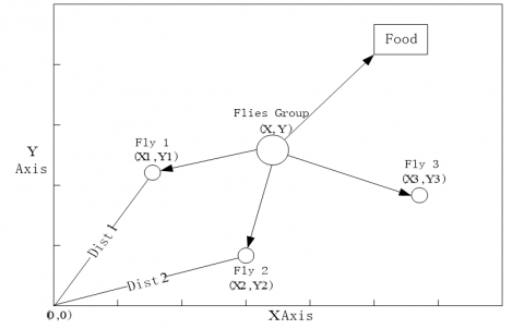
Fruit fly optimization algorithm (FOA) is a new swarm intelligence method, which was proposed by Pan (2012). The FOA is a new method for finding global optimization based on the food finding behavior of the fruit fly. The fruit fly is superior to other species in vision and osphresis. The food finding process of fruit fly is as follows: firstly, it smells the food source by osphresis organ, and flies towards that location; then, after it gets close to the food location, the sensitive vision is also used for finding food and other fruit flies’ flocking location, and it flies towards that direction. Figure 1 shows the food finding iterative process of fruit fly swarm.
Figure 1. Food finding iterative process of fruit fly swarm
In this paper, based on the food finding characteristics of the fruit fly, it is divided into several necessary steps, just as followings:
Step 1: The main parameters of the FOA are the maximum iteration number maxgen, the population sizepop and the initial fruit fly swarm location as bellows:
$Init\begin{matrix} {} \\\end{matrix}X\_axis$ (12)
$Init\begin{matrix} {} \\\end{matrix}Y\_axis$ (13)
Step 2: Give the random direction and distance for the search of food using osphresis by an individual fruit fly.
${{X}_{i}}=X\_axis+RandomValue$ (14)
${{Y}_{i}}=Y\_axis+RandomValue$ (15)
Step 3: Since the food location cannot be known, the distance to the origin is thus estimated first (Dist), then the smell concentration judgment value (S) is calculated, and this value is the reciprocal of distance.
$Dis{{t}_{i}}=\sqrt{X_{i}^{2}+Y_{i}^{2}}$ (16)
${{S}_{i}}=\frac{1}{Dis{{t}_{i}}}$ (17)
Step 4: Substitute smell concentration judgment value (S) into smell concentration judgment function (or called Fitness function) so as to find the smell concentration (Smelli) of the individual location of the fruit fly.
$Smel{{l}_{i}}=Function({{S}_{i}})$ (18)
Step 5: Find out the fruit fly with maximal smell concentration (finding the maximal value) among the fruit fly swarm.
$[bestSmell\begin{matrix} {} \\\end{matrix}bestIndex]=\max (Smell)$ (19)
Step 6: Keep the best smell concentration value and x, y coordinate. At this moment, the fruit fly swarm will use vision to fly towards that location.
$Smellbest=bestSmell$ (20)
$X\_axis=X(bestIndex)$ (21)
$Y\_axis=Y(bestIndex)$ (22)
Step 7: Enter iterative optimization to repeat the implementation of Steps 2-5, then, judge if the smell concentration is superior to the previous iterative smell concentration, if so, implement the Step 6.
FOA belongs to a kind of interactive evolutionary computation, and also is a part of the artificial intelligence. Therefore, it has been widely applied to solve the problems in military, engineering, management and financial affairs.
3.3. Fruit fly optimization algorithm for the parameters selection of the LSSVM model
Figure 2. The flowchart of the FOALSSVM model
Selecting appropriate values of the kernel function
and penalty coefficient are particularly important. In this paper, the FOA was used for selecting the suitable parameter values of the LSSVM model in order to effectively improve the short-term photovoltaic power forecasting accuracy.The flowchart of the FOA for the parameters of the LSSVM model (abbreviated as FOALSSVM) is shown in Figure 2.
The details of the FOALSSVM are shown as follows:
Step 1: Initialization parameters.
The maximum iteration number maxgen, the population size sizepop, the initial fruit fly swarm location (X_axis, Y_axis), and the random flight distance range FR should be determined at first. In this paper, suppose maxgen=100, sizepop=10,
and .Step 2: Evolution starting.
Set gen=0, and give the random flight direction and the distance for food finding of an individual fruit fly.
Step 3: Preliminary calculation.
Calculate the flight distance Disti of the fruit fly i, and then calculate the smell concentration judgment value Si. Input Si into the LSSVM model for the short-term photovoltaic power forecasting. According to the result of photovoltaic power forecasting, calculate the smell concentration Smelli (also called the fitness function value). The Smelli is employed the root-mean-square-error (RMSE) which measures the deviation between the forecasting value and the actual value.
$\left\{ \begin{matrix} \gamma =20*\max ({{S}_{i}}) \\ \sigma =\min ({{S}_{i}}) \\\end{matrix} \right.$ (23)
$RMSE=\sqrt{\frac{\sum\limits_{i=1}^{n}{{{(P_{i}^{r}-P_{i}^{f})}^{2}}}}{n}}$ (24)
where
and are the actual and training output power of PV power station, respectively; n is the number of training sample.Step 4: Offspring generation.
The offspring generation is generated according equation (12) to equation (22). Then input the offspring into the LSSVM model and calculate the smell concentration value again. Set gen=gen+1.
Step 5: Circulation stops.
When gen reaches the max iterative number, the stop criterion satisfies, and the best parameter values of the LSSVM model can be obtained. Otherwise, go back to Step 2.
In this paper, the FOALSSVM algorithm was simulated by the MATLAB and one demonstration project of PV power generation in Jiangsu province was selected to prove the effectiveness of the proposed FOALSSVM algorithm.
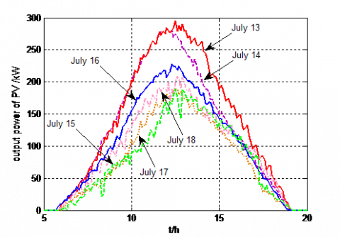
The capacity of PV power generation system is 380 kW. It was chosen the local meteorological data and historical output power of PV generation as the training sample in July, then forecasted the someday output power of PV generation in step size of 15 minutes. As shown in Figure 3, it is provided the output power curves of PV power generation from July 13th to July 18th.
Figure 3. Curves of PV power generation data
The operation curves of PV generation show that the effective working period of PV generation is from about 6 o’clock in the morning to 19 o’clock in the afternoon, while the output power of PV generation is zero in the rest time of a day. Therefore, the output power forecasting of PV generation can be only restricted in the working period.
The procedures for applying the proposed FOALSSVM algorithm to forecast the output power of PV generation are described as follows:
Step 1: The process of sample data.
In this paper, the sample data were normalized to make data in the range from 0 to 1 using the following formula:
$X=\frac{{{x}_{i}}-{{x}_{i\min }}}{{{x}_{i\max }}-{{x}_{i\min }}},i=1,2,\cdots ,l$ (25)
where ximax and ximin are the maximal and minimal value of each input factor, respectively.
Step 2: Train the LSSVM model.
In the FOALSSVM model, the parameter values of the LSSVM are dynamically tuned by the FOA. The initial parameter values of the LSSVM were set up in the range of [0.01, 1]. After 100 times of iterative evolution, the optimal parameter values of the LSSVM are obtained in Table 1.
Table 1. The parameter values of the three algorithms
|
Parameter |
SVM |
LSSVM |
FOALSSVM |
|
$\sigma$ |
0.2 |
0.5 |
0.18 |
|
$\gamma$ |
1 |
10 |
5.48 |
Step 3: Forecast the output power of PV generation.
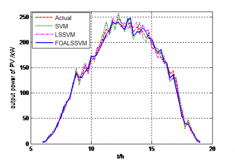
According to the result of FOA tuning the parameters of the LSSVM model, the parameters of kernel function $\sigma$ and penalty coefficient $\gamma$ are chosen as 0.18 and 5.48 to forecast the output power of PV generation, respectively. The final forecasted output power of PV generation is shown in Figure 4 and Table 2.
It was taken the historical output power data and the predictive meteorological of the day as input to forecast the output power of July 19th in per 15 minutes, and compared with the actual output power of PV generation station. The absolute percentage error (APE) and mean absolute percentage error (MAPE) are adopted to analyze and measure the performance of the forecasting models in the PV power forecasting, which can be calculated by:
${{\varepsilon }_{APE}}=\frac{\left| {{Y}_{r}}-{{Y}_{e}} \right|}{{{Y}_{r}}}\times 100%$ (26)
${{\varepsilon }_{MAPE}}=\frac{1}{n}\sum\limits_{i=1}^{n}{{{\varepsilon }_{APE}}}$ (27)
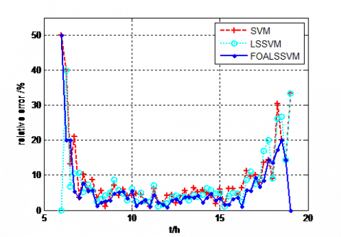
Table 2 shows the forecasting results of PV generation by the SVM, LSSVM and FOALSSVM algorithms in per 15 minutes, respectively. Among of them, the MAPE of short-term PV power forecasting based on FOALSSVM is 6.32%, while the values based on SVM and LSSVM are 8.93% and 7.67%, respectively. Figure 4 gives the forecasting results with the SVM, LSSVM and FOALSSVM algorithms. Figure 5 describes the error analysis of the three forecasting algorithms.
Figure 4. PV power forecasting results curves
Table 2. The forecasting results with the SVM, LSSVM and FOALSSVM algorithms
|
Time |
Actual value (kW) |
SVM |
LSSVM |
FOALSSVM |
|||
|
Result (kW) |
Error (%) |
Result (kW) |
Error (%) |
Result (kW) |
Error (%) |
||
|
6:00 |
2 |
3 |
50.0 |
2 |
0.0 |
3 |
50.0 |
|
6:15 |
5 |
7 |
40.0 |
7 |
40.0 |
6 |
20.0 |
|
6:30 |
15 |
13 |
13.3 |
16 |
6.7 |
12 |
20.0 |
|
6:45 |
19 |
23 |
21.1 |
17 |
10.5 |
18 |
5.3 |
|
7:00 |
28 |
29 |
3.6 |
25 |
10.7 |
27 |
3.6 |
|
7:15 |
39 |
35 |
10.3 |
37 |
5.1 |
42 |
7.7 |
|
7:30 |
55 |
58 |
5.5 |
59 |
7.3 |
52 |
5.5 |
|
7:45 |
69 |
63 |
8.7 |
65 |
5.8 |
73 |
5.8 |
|
8:00 |
83 |
80 |
3.6 |
85 |
2.4 |
82 |
1.2 |
|
8:15 |
90 |
95 |
5.6 |
87 |
3.3 |
92 |
2.2 |
|
8:30 |
115 |
114 |
1.0 |
120 |
4.3 |
118 |
2.6 |
|
8:45 |
142 |
148 |
4.2 |
135 |
4.9 |
138 |
2.8 |
|
9:00 |
125 |
116 |
7.2 |
136 |
8.8 |
131 |
4.8 |
|
… |
… |
… |
… |
… |
… |
… |
… |
|
17:15 |
88 |
95 |
8.0 |
80 |
9.1 |
82 |
6.8 |
|
17:30 |
59 |
67 |
13.6 |
69 |
17.0 |
54 |
8.5 |
|
17:45 |
35 |
30 |
14.3 |
42 |
20.0 |
40 |
14.3 |
|
18:00 |
44 |
48 |
9.1 |
40 |
9.1 |
38 |
13.6 |
|
18:15 |
23 |
30 |
30.4 |
29 |
26.1 |
27 |
17.4 |
|
18:30 |
15 |
12 |
20.0 |
19 |
26.7 |
18 |
20.0 |
|
18:45 |
7 |
6 |
14.3 |
6 |
14.3 |
8 |
14.3 |
|
19:00 |
3 |
4 |
33.3 |
2 |
33.3 |
3 |
0.0 |
Figure 5. Error curves based on different algorithms
From the forecasting results we reach the following conclusions:
(1) It can be clearly seen that all the three forecasting algorithms capture the output trends of the PV generation, but the performance of FOALSSVM algorithm is better than the others.
(2) From the 6 to 8 o’clock in the morning, the forecasting errors are relatively larger. Because of the humidity has an effect on the PV power generation system, the curve of output power is unstable. However, there is obvious correlation between the human body amenity and humidity, which causes the good forecasting performance by the FOALSSVM in this time quantum.
(3) In the afternoon, the PV generation is covered by a part of cloud, which leads the output power of PV generation in high volatility. Therefore, there exist larger deviations between the forecasting results and the actual output.
Generally speaking, the proposed human body amenity and FOALSSVM algorithm can narrow the deviation between the forecasting results and the actual values, and it outperforms the SVM and LSSVM algorithm in the short-term PV power forecasting. Compared with the LSSVM algorithm, the FOALSSVM which uses the FOA to select the parameter values of the LSSVM can improve the forecasting accuracy effectively.
The LSSVM algorithm has been widely used in variety of fields, but it rarely finds that the LSSVM have been applied to the PV power forecasting. In this paper, a hybrid model based on human body amenity and LSSVM with FOA were proposed for the short-term PV power forecasting. The human body amenity can effectively use the various meteorological factors, reduce the input of network and improve the precision of forecasting. Meanwhile, the FOALSSVM model uses the FOA to automatically select the appropriate parameter values of LSSVM in order to improve the forecasting accuracy. For comparison, another two models such as SVM and LSSVM were selected. The simulating results show: the FOA can select the appropriate parameter values of the LSSVM model, which could effectually improve the forecasting accuracy of PV output power. Compared with the SVM and LSSVM algorithm, the values of APE and MAPE are obviously smaller than that of other two algorithms.
This work is supported by Graduate Education Innovation Project in Jiangsu Province (No.CXZZ12_0228) and the Jiangsu Science and Technology Planning Project (BE2012014). The authors would like to thank the editor and anonymous reviewers for their suggestions in improving the quality of the paper.
Ai-Hamadi H. M., Soliman S. A. (2005). Long-term/mid-term electric load forecasting based on short-term correlation and annual growth. Electric Power Systems Research, Vol. 74, No. 3, pp. 353-361. https://doi.org/10.1016/j.epsr.2004.10.015
Almonacid F., Rus C., Perez P. J., Hontoria L. (2009). Estimation of the energy of a PV generator using artificial neural network. Renewable Energy, Vol. 34, No. 12, pp. 2743-2750. https://doi.org/10.1016/j.renene.2009.05.020
Benghanem M., Mellit A., Alamri S. N. (2009). ANN-based modeling and estimation of daily global solar radiation data: A case study. Energy Conversation Management, Vol. 7, No. 1, pp. 1644-1655. https://doi.org/10.1016/j.jclepro.2016.09.145
Cortes C., Vapnik V. (1995). Support-vector networks. Machine Learning, Vol. 20, No. 3, pp. 273-297. https://doi.org/10.1007/BF00994018
Damousis I. G., Bakirtzis A. G., Dokopoutos P. S. (2004). A solution to the unit-commitment problem using integer-coded genetic algorithm. IEEE Transactions on Power Systems, Vol. 19, No. 2, pp. 1165-1172. https://doi.org/10.1109/TPWRS.2003.821625
Du Y., Lu J. P., Li Q., Deng Y. L. (2008). Short-term wind speed forecasting of wind farm based on least square-support vector machine. Power System Technology, Vol. 32, No. 15, pp. 62-66. https://doi.org/10.1109/CCECE.2010.5575154
Hsu C. C., Chen C. Y. (2003). Regional load forecasting in Taiwan–applications of artificial neural networks. Energy Conversion and Management, Vol. 44, No. 12, pp. 1941-1949. https://doi.org/10.1016/s0196-8904(02)00225-x
Keerthi S. S., Lin C. J. (2003). Asymptotic behaviors of support vector machines with Gaussian kernel. Neural Computation, Vol. 15, No. 1, pp. 1667-1689. https://doi.org/10.1162/089976603321891855
Lu N., Qin J., Yang K., Sun J. (2011) A simple and efficient algorithm to estimate daily global solar radiation from geostationary satellite data. Energy, Vol. 5, No. 1, pp. 3179-3188. https://doi.org/10.1016/j.energy.2011.03.007
Mellit A., Pavan A. M. (2010). Performance prediction of 20 kW grid-connected photovoltaic plant at Trieste (Italy) using artificial neural network. Energy Conversion and Management, Vol. 51, No. 1, pp. 2431-2441. https://doi.org/10.1016/j.enconman.2010.05.007
Pai P. F., Hong W. C. (2005). Support vector machines with simulated annealing algorithms in electricity load forecasting. Energy Conversion and Management, Vol. 46, No. 17, pp. 2669-2688. https://doi.org/10.1016/j.enconman.2005.02.004
Pan W. T. (2012). A new fruit fly optimization algorithm: taking the financial distress as an example. Knowledge-Based Systems, Vol. 26, No. 2, pp. 69-74. https://doi.org/10.1016/j.knosys.2011.07.001
Qin H. C., Wang W., Zhou H., Wang L. (2006). Short-term electric load forecast using human body amenity indicator. Proceedings of the CSU-EPSA, Vol. 18, No. 2, pp. 63-66. https://doi.org/10.1049/cp.2015.0550
Rehman S., Mohandes M. (2008). Artificial neural network estimation of global solar radiation using air temperature and relative humidity. Energy Policy, Vol. 2, No. 1, pp. 571-576. https://doi.org/10.1016/j.enpol.2007.09.033
van Gestel T., Suykens J. A. K., Baesens B., Viaene S., Vanthienen J., Dedene G., Moor B., Candewalle J. (2004). Benchmarking least squares support vector machine classifiers. Machine Learning, Vol. 54, No. 1, pp. 5-32. https://doi.org/10.1023/B:MACH.0000008082.80494.e0
Wang F., Mi Z., Su S., Zhao H. (2012). Short-term solar irradiance forecasting model based on artificial neural network using statistical feature parameters. Energies, Vol. 5, No. 1, pp. 1355-1370. https://doi.org/10.3390/en5051355
Yorukoglu M., Celik A. N. (2006). A critical review on the estimation of daily global solar radiation from sunshine duration. Energy Conversation Management, Vol. 15, No. 1, pp. 2441-2450. https://doi.org/10.1016/j.enconman.2005.11.002
Zhu Y. Q., Tian J. (2011). Application of least square support vector machine in photovoltaic power forecasting. Power System Technology, Vol. 35, No. 7, pp. 54-59. https://doi.org/10.3354/cr00999