Hesna Aberkane* | Djamel Sakri | Djamel Rahem
© 2021 IIETA. This article is published by IIETA and is licensed under the CC BY 4.0 license (http://creativecommons.org/licenses/by/4.0/).
OPEN ACCESS
Induction motors (IM) are widely used in power industry applications, many efforts have been made to enhance their energy efficiency and to reduce environmental pollution for these last reasons, different control techniques have been developed, among them, conventional predictive torque control (PTC) is based on the principle of keeping a constant stator reference flux independently of operating point, such situation generates significant losses and reduces the performance especially when the machine is lightly loaded. In order to maximize induction motor energy performance, the present research proposes an optimization of predictive torque control (OPTC) strategy, based on induction motor loss model (LMC). The aim of LMC technique is to deduce the best flux references to apply to the induction machine in order to minimize the copper and iron losses therefore improve the motor efficiency. So to confirm the theoretical study, experimental tests for various operating conditions of IM are proposed to verify the efficacy of the proposed OPTC. The obtained results show that OPTC decreases the total IM drive losses and ensures a significant increase in efficiency especially when the motor operates outside nominal conditions.
direct torque control, induction motor, loss model, optimized predictive torque control, predictive torque control
Electrical energy consumption continues to grow in the world. Statistics show that the electric drives consume more than 56% of the energy for the variable speed sector, where 96% of them are consumed directly by induction motors, which means that almost 53% of the totality electrical energy is consumed by this type of motors. This wide use of induction motors in various industry applications is effectively justified by their well-known intrinsic properties such as: low cost, robustness and simplicity of construction and overloads supporting up to 7 times their nominal torque [1].
Nowadays, improving induction motors energy performance is becoming a big challenge for researchers around the world. The objectives are doubled; economic and environmental (pollution reduction).
Generally, the energy performance improvement and minimization of the induction motors losses is carried out either by: the judicious choice of the material or the choice of an optimal control technique. In this paper a predictive torque control (PTC) method based on losses model control (LMC) used as an optimal control technique.
Generally, the control of induction motor is difficult because of the strong coupling between stator and rotor quantities (speed, torque and flux), the efficiency and power factor can be damaged when the IM is lightly loaded. However, the IM requires more control performances: accurate and fast torque and flux response, large torque at low speed, wide speed range, the drive control system is necessary for IM [2].
Thanks to the advancements of power electronics and computer tools, various control methods were developed, such as scalar control, field oriented control, direct torque control. In the last decades, the direct torque control (DTC) has become a popular technique for three-phase induction motor (IM) drives because it provides a fast dynamic torque response and robustness under machine parameter variations without the use of current regulators [3], the direct torque control (DTC) method was proposed for the conduct of IM by Depenbrock and Takahashi. DTC is known to produce a robust and a fast response in AC drives [4, 5]. However, remarkable torque and current ripples occur [6]. The DTC topology consists directly to control the stator flux and electromagnetic torque separately and keeps them within their hysteresis band from the hysteresis regulators [7], which are the principal sources of the ripple appearing at the current and the torque due to their variable switching frequency [8-10], and it also consists of a switching table to select the voltage vector applied to the motor [11].
Recently, predictive torque control (PTC) strategy has received wide attention in research communities due to their intuitive features, simple implementation, easy inclusion of nonlinearities, design constraints [12, 13], and straightforward implementation. Furthermore, the system constraints can be easily considered by a cost function. The PTC uses the inherent discrete nature of the power converter to solve the optimization problem using a single cost function. The cost function chooses the control inputs from a restricted finite set of discrete values. The discrete system model is evaluated for every possible actuation sequence and then compared with the reference in order to select the best voltage vector [14].
The main objective of this paper is to achieve a high IM control performance and to decrease the electromagnetic losses. The proposed OPTC strategy is based on the association of losses model control method (LMC) which generates the optimal stator flux reference with the finite set predictive torque control (FS-PTC). The optimal stator flux reference is generated by minimizing the IM total losses cost function, in order to obtain the maximum efficiency. The generated stator flux reference is feed to finite set PTC, which in turn, generates the optimal inverter control signal in order to minimize the torque and flux tracking errors. Finally, several experimental tests obtained by a DSPACE 1104 card, were carried out to validate the feasibility of the proposed method.
The mathematical model of induction motor in a fixed stator reference frame (α, β) can be described by the following equations [15]:
$\left\{ \begin{align} & \frac{d{{i}_{s\alpha }}}{dt}=-{{a}_{1}}{{i}_{s\alpha }}-{{a}_{2}}{{\psi }_{r\alpha }}+\frac{{{\omega }_{r}}}{\sigma {{L}_{s}}(1+{{\sigma }_{r}})}{{\psi }_{r\beta }}+\frac{1}{\sigma {{L}_{s}}}{{v}_{s\alpha }} \\ & \frac{d{{i}_{s\beta }}}{dt}=-{{a}_{1}}{{i}_{s\beta }}-{{a}_{2}}{{\psi }_{r\beta }}-\frac{{{\omega }_{r}}}{\sigma {{L}_{s}}(1+{{\sigma }_{r}})}{{\psi }_{r\alpha }}+\frac{1}{\sigma {{L}_{s}}}{{v}_{s\beta }} \\ & \frac{d{{\psi }_{r\alpha }}}{dt}={{a}_{3}}{{i}_{s\alpha }}-{{a}_{4}}{{\psi }_{r\alpha }}-{{\omega }_{r}}{{\psi }_{r\beta }} \\ & \frac{d{{\psi }_{r\beta }}}{dt}={{a}_{3}}{{i}_{s\beta }}-{{a}_{4}}{{\psi }_{r\beta }}+{{\omega }_{r}}{{\psi }_{_{r\alpha }}} \\\end{align} \right.$ (1)
where:
$\begin{align} & {{a}_{1}}=\frac{{{R}_{s}}}{\sigma {{L}_{s}}}+\frac{{{\sigma }_{r}}{{R}_{fs}}}{\sigma {{L}_{s}}(1+{{\sigma }_{r}})}+\frac{{{R}_{f}}-{{\sigma }_{r}}{{R}_{fr}}}{\sigma {{L}_{s}}{{(1+{{\sigma }_{r}})}^{2}}}, \\ & {{a}_{2}}=\frac{{{R}_{fs}}}{\sigma {{L}_{s}}{{L}_{r}}}\frac{{{R}_{f}}+{{R}_{fs}}}{\sigma {{L}_{s}}(1+{{\sigma }_{r}})} \\ & {{a}_{3}}=\frac{{{R}_{f}}-{{\sigma }_{r}}{{R}_{fr}}}{(1+{{\sigma }_{r}})},{{a}_{4}}=\frac{{{R}_{f}}+{{R}_{fr}}}{{{L}_{r}}} \\\end{align}$${{\sigma }_{r}}=\frac{{{l}_{r}}}{M},{{\sigma }_{s}}=\frac{{{l}_{s}}}{M},\sigma =1-\frac{{{M}^{2}}}{{{L}_{s}}{{L}_{r}}}$ (2)
And
$\begin{align} & {{R}_{fs}}={{K}_{e}}{{f}^{2}}+{{K}_{h}}f \\ & {{R}_{fr}}=g{{K}_{e}}{{f}^{2}}+g{{K}_{h}}f \\\end{align}$ (3)
The IM mechanical equation is given by:
$J\frac{d\Omega }{dt}=T-f\Omega -{{T}_{L}}$ (4)
With:
$T=\frac{pM}{{{L}_{r}}}\left( {{\psi }_{r\alpha }}{{i}_{s\beta }}-{{\psi }_{r\beta }}{{i}_{s\alpha }} \right)$ (5)
And ${{T}_{L}}$ is the load torque.
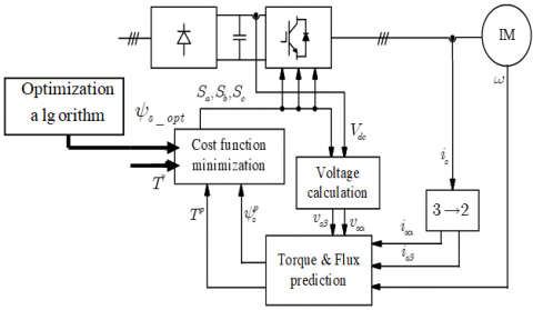
The mathematical model of a two-level voltage inverter, presented in Figure 1, is given by:
$\left[\begin{array}{c}V_{a n} \\ V_{b n} \\ V_{c n}\end{array}\right]=\frac{V_{d c}}{3}\left[\begin{array}{ccc}2 & -1 & -1 \\ -1 & 2 & -1 \\ -1 & -1 & 2\end{array}\right]\left[\begin{array}{c}S_{a} \\ S_{b} \\ S_{c}\end{array}\right]$ (6)
Figure 1. 2L-VSI fed induction motor
Model predictive control shown in Figure 2 is constituted by the prediction models of the stator flux, electromagnetic torque and the cost function, while the predictive values of stator flux and the torque are obtained using the prediction models. Compared to the conventional DTC, the outer loop of the PTC is also a speed loop, and the reference torque is obtained from a PI regulator. The main difference between the two control methods is that the inner loop of the PTC employs a model predictive controller instead of the stator flux and torque hysteresis comparators used in the conventional DTC. The PTC is based on three steps: estimation, prediction and cost function minimization, [12, 16]. The inverter model is directly considered in the PTC method. All feasible switching vectors are calculated for the optimum selection. A cost function is built for the best switching signals selection. In this system, the performance required computational of the modular analyzed for a two-level voltage source inverter (2L-VSI), it is well known that a 2L-VSI produces eight voltage vectors {v0…v7} [13].
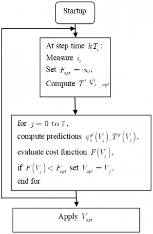
The synoptic control and the flowchart of PTC are illustrated in Figure 2 and Figure 3:
Figure 2. PTC control diagram
Figure 3. PTC flowchart
The prediction is computed for the eight possible voltage vector Vs and the cost function selects the voltage vector that produces the best flux and torque control.
The cost function is defined as [14]:
$F=\left| {{T}^{*}}-{{T}^{p}}(k+1) \right|+\tfrac{{{T}_{n}}}{{{\psi }_{n}}}\left| \psi _{s}^{*}-\psi _{s}^{p}(k+1) \right|$ (7)
where:
${{T}^{*}},{{T}^{p}}(k+1)$: Reference and predicted torque.
$\psi _{s}^{*},\psi _{s}^{p}(k+1)$ : Reference and predicted stator flux.
Generally, the model of IM is used for Current, flux and torque predictions can be expressed in discrete time steps as following [13]:
Current prediction:
$\left\{ \begin{align} & i_{s\alpha }^{p}(k+1)={{i}_{s\alpha }}\left( k \right)+{{T}_{s}}(-{{a}_{1}}{{i}_{s\alpha }}\left( k \right)-{{a}_{2}}{{\psi }_{r\alpha }}\left( k \right)+ \\ & \,\,\,\,\,\,\,\,\,\,\,\,\,\,\,\,\,\,\,\,\,\,\,\,\frac{{{\omega }_{r}}\left( k \right)}{\sigma {{L}_{s}}(1+{{\sigma }_{r}})}{{\psi }_{r\beta }}\left( k \right)+\frac{1}{\sigma {{L}_{s}}}{{v}_{s\alpha }}\left( k \right)) \\ & i_{s\beta }^{p}(k+1)={{i}_{s\alpha }}\left( k \right)+{{T}_{s}}(-{{a}_{1}}{{i}_{s\beta }}\left( k \right)-{{a}_{2}}{{\psi }_{r\beta }}\left( k \right) \\ & \,\,\,\,\,\,\,\,\,\,\,\,\,\,\,\,\,\,\,\,\,\,\,\,\,-\frac{{{\omega }_{r}}\left( k \right)}{\sigma {{L}_{s}}(1+{{\sigma }_{r}})}{{\psi }_{r\alpha }}\left( k \right)+\frac{1}{\sigma {{L}_{s}}}{{v}_{s\beta }}\left( k \right)) \\\end{align} \right.$ (8)
Rotor flux prediction:
$\left\{ \begin{align} & \psi _{r\alpha }^{p}(k+1)={{a}_{3}}{{T}_{e}}i_{s\alpha }^{p}(k+1)-({{T}_{e}}{{a}_{4}}-\frac{1}{{{T}_{e}}}){{\psi }_{r\alpha }}(k) \\ & \,\,\,\,\,\,\,\,\,\,\,\,\,\,\,\,\,\,\,-{{\psi }_{r\beta }}(k){{T}_{e}} \\ & \psi _{r\beta }^{p}(k+1)={{a}_{3}}{{T}_{e}}i_{s\beta }^{p}(k+1)-({{T}_{e}}{{a}_{4}}-\frac{1}{{{T}_{e}}}){{\psi }_{r\beta }}(k) \\ & \,\,\,\,\,\,\,\,\,\,\,\,\,\,\,\,\,\,+{{\omega }_{r}}{{\psi }_{r\alpha }}(k){{T}_{e}} \\\end{align} \right.$ (9)
Stator flux prediction:
$\left\{ \begin{align} & \psi _{s\alpha }^{p}(k+1)=\sigma {{L}_{s}}i_{s\alpha }^{p}(k+1)+\frac{M}{{{L}_{r}}}\psi _{r\alpha }^{p}(k+1) \\ & \psi _{s\beta }^{p}(k+1)=\sigma {{L}_{s}}i_{s\beta }^{p}(k+1)+\frac{M}{{{L}_{r}}}\psi _{r\beta }^{p}(k+1) \\\end{align} \right.$ (10)
Torque prediction:
$\begin{align} & {{T}^{p}}(k+1)=p(\psi _{s\alpha }^{p}(k+1)i_{s\beta }^{p}(k+1) \\ & \,\,\,\,\,\,\,\,\,\,\,\,\,\,\,\,\,\,-\psi _{s\beta }^{p}(k+1)i_{s\alpha }^{p}(k+1)) \\\end{align}$ (11)
In PTC topology, the stator reference flux is constant [10]; this situation generates important losses and decreases the performances of IM especially when it is lightly loaded. So to avoid this problem and to optimize the energy performance, and consequently to minimize the losses of the PTC strategy, an algorithm based on losses model has been introduced to generate the reference flux. The new method named optimized predictive torque control ‘OPTC’.
On the energy side, it is well known that IM has a good performance when it works around the nominal point and deteriorates outside this point of operation [17]. The PTC control considers a constant stator flux reference [18, 19] thus independent of the states of the machine. Such a situation generates important losses in the IM and consequently the efficiency was decreased [1].
According to the IM per phase equivalent circuit, the total losses can be evaluated as:
$P_{l o s s}=3 R_{s} i_{s}^{2}+3 R_{r} i_{r}^{2}+R_{f s} i_{s \alpha}^{2}+\frac{\sigma_{r}}{\left(1+\sigma_{r}\right)} R_{f s} i_{s \beta}^{2}$ (12)
Loss Model Control "LMC" approach is based on analytical calculation of the optimal flux which the objective function of the losses was minimal, while considering the operating conditions such as speed and the torque [1, 20].
The loss function (${{P}_{loss}}$) will be defined as:
$\begin{align} & {{P}_{loss}}=\frac{({{R}_{s}}+{{R}_{fs}})}{{{M}^{2}}}\psi _{r\alpha }^{2}+ \\ & \,\,\,\,\,\,\left[ \frac{{{R}_{s}}+\frac{{{R}_{r}}}{{{(1+{{\sigma }_{r}})}^{2}}}+\frac{{{\sigma }_{r}}\,{{R}_{fs}}}{(1+{{\sigma }_{r}})}}{{{(p(1-\sigma )(1+{{\sigma }_{s}}))}^{2}}} \right]{{T}^{2}}\psi _{r\beta }^{-2} \\\end{align}$ (13)
Therefore, in order to minimize losses, and optimize efficiency, an algorithm for generating the flux will be proposed. The principle of this optimization strategy is to generate the optimal rotor flux by the LMC technique and finally to deduce the stator.
According to references, [18], the stator and rotor flux are defined by the following relation:
$\left\{ \begin{align} & {{\psi }_{s\alpha }}=\frac{{{L}_{s}}}{M}{{\psi }_{r}}+\frac{\sigma {{L}_{s}}{{L}_{r}}}{{{R}_{r}}M}\frac{d{{\psi }_{r}}}{dt} \\ & {{\psi }_{s\beta }}=\frac{2}{3}\frac{\sigma {{L}_{s}}{{L}_{r}}}{pM}\frac{T}{{{\psi }_{r}}} \\\end{align} \right.$ (14)
In steady status:
${{\psi }_{r}}=\left| \overline{{{\psi }_{r}}} \right|={{\psi }_{r\_opt}}$ (15)
where:
${{\psi }_{r\_opt}}={{Y}_{opt}}{{(\left| {{T}^{*}} \right|)}^{\frac{1}{2}}}$ (16)
With:
${{Y}_{opt}}={{\left[ \begin{align} & \frac{M}{p(1-\sigma )(1+{{\sigma }_{s}})}* \\ & {{\left[ \frac{{{R}_{s}}+\frac{{{R}_{r}}}{{{(1+{{\sigma }_{r}})}^{2}}}+\frac{{{\sigma }_{r}}{{R}_{fs}}}{(1+{{\sigma }_{r}})}}{{{R}_{s}}+{{R}_{fs}}} \right]}^{\frac{1}{2}}} \\\end{align} \right]}^{\frac{1}{2}}}$ (17)
From the flowing equation:
$\begin{align} & {{\left( \psi _{s}^{*} \right)}^{2}}={{\left( \psi _{s\alpha }^{*} \right)}^{2}}+{{\left( \psi _{s\beta }^{*} \right)}^{2}} \\ & ={{\left( \frac{{{L}_{s}}}{M}\psi _{r}^{*} \right)}^{2}}+{{\left( \frac{2}{3}\frac{\sigma {{L}_{s}}{{L}_{r}}}{pM} \right)}^{2}}{{\left( \frac{{{T}^{*}}}{\psi _{r}^{*}} \right)}^{2}} \\\end{align}$ (18)
The reference flux, required by an OPTC method, is defined as a function of the rotor flux reference and the torque [20, 21]. The optimal stator flux can be deduced as:
${{\psi }_{s\_opt=\frac{{{L}_{s}}}{M}}}\sqrt{{{\left( {{\psi }_{r\_opt}} \right)}^{2}}+{{\left( \frac{2}{3}\frac{\sigma {{L}_{r}}}{p} \right)}^{2}}{{\left( \frac{{{T}^{*}}}{{{\psi }_{r\_opt}}} \right)}^{2}}}$ (19)
Figure 4. OPTC control diagram
Figure 5. OPTC flowchart
So, in classical PTC, the stator flux was maintained to its nominal value, however in the OPTC method, stator flux was variable and dependent to the load variation.
The block diagram of the OPTC and the flowchart explaining its different steps are given respectively by Figure 4 and Figure 5.
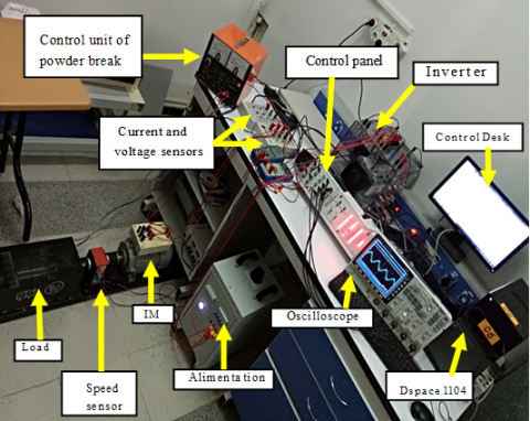
The PTC and OPTC algorithms were tested experimentally on the test bench shown by the photography on Figure 6, which is based on:
- DSPACE 1104 card for the real-time implementation of predictive torque control in its two versions, classic and optimized, which ensures the digital aspect of the control from the digital acquisition of the input signals to the control output signals by using of a control desk interface which makes it possible to view in real time various variables.
- Three-phase squirrel cage induction motor (IM). Its windings are star-coupled, with the following nominal values: $\left(P_{n}=1.5 K W, I_{n}=3.4 / 5.9 A, N_{n}=1423 r p / m\right)$, the motor is fed by a controlled 2L-VSI from SEMKRON, with a variable three-phase voltage source (0 to 450V).
- Powder brake was used as a load and can be controlled manually or externally via a computer.
The tests carried out consist in varying the load torque from 1 Nm to 4 Nm while maintaining the speed equal to 1000 rp/m. For several operating points, a switching test is made between PTC (classic model) and OPTC (based on LMC model) algorithms in order to see the optimization effect.
All the experimental results are saved in a (.mat) file then plotted by the Matlab-Simulink software.
Figure 6. Experimental setup for PTC & OPTC
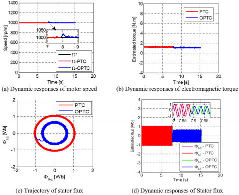
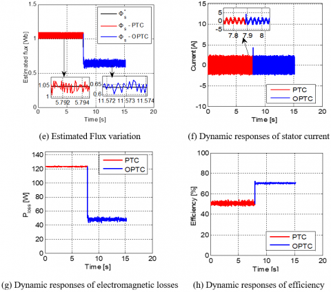
For the first test, IM is exposed to a load torque of 1 Nm. The analysis of the curves of Figure 7, allows us to make the following comments:
• Speed, torque and stator current reach their references without being affected by the switching.
• When the switching test is applied, a reduction of stator flux level is very, representing the circular trajectory and time evolution of stator flux. This is justified by the optimization algorithm that depends on the operating point.
• For curves interpreting the energy balance, a significant minimization of the total losses of the motor is obtained at the time of switching, which brings an improvement of the motor efficiency.
For all the other tests, both PTC and OPTC offer a fast dynamic response for speed, electromagnetic torque, stator current, all this signals are independent of load variation, so the optimization has no effect on them.
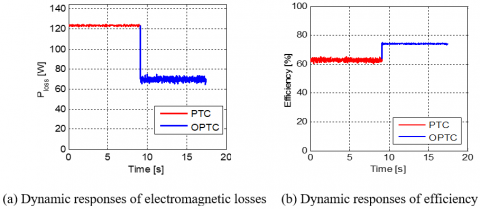
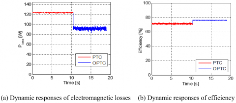
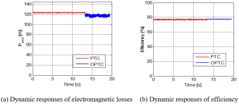
Figure 8, Figure 9 and Figure 10, presents the energetic behavior (electromagnetic losses and efficiency) of the two methods have been studied according to different values of the load torque (TL=2N.m, TL=3N.m and TL=4N.m).
Figure 7. Performance comparison of PTC and proposed OPTC for TL=1N.m
Figure 8. Performance comparison of PTC and proposed OPTC for TL=2N.m
Figure 9. Performance comparison of PTC and proposed OPTC for TL=3N.m
Figure 10. Performance comparison of PTC and proposed OPTC for TL=4N.m
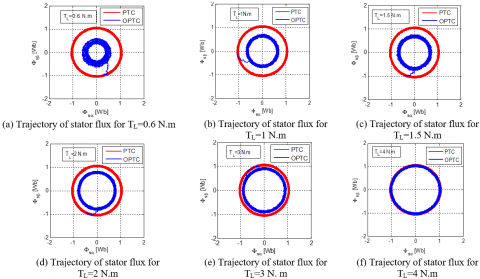
Figure 11. Stator flux trajectory evolution for PTC and OPTC
Table 1. Summary PTC and OPTC optimization for experimental results
|
${{\text{T}}_{\text{L}}}\text{(N}\text{.m)}$ |
${{\psi }_{s}}\text{(Wb)}$ |
${{\text{P}}_{\text{loss }}}\text{(W)}$ |
$\eta(\%)$ |
|||
|
|
PTC |
OPTC |
PTC |
OPTC |
PTC |
OPTC |
|
1 |
1.05 |
0.5 |
125 |
40 |
40 |
68 |
|
2 |
1.05 |
0.7 |
123 |
70 |
50 |
70 |
|
3 |
1.05 |
0.9 |
122 |
100 |
60 |
70 |
|
4 |
1.05 |
1 |
122 |
115 |
68 |
70 |
According to the Table 1, summarizing the results of the test, when the speed is kept constant equal to 1000 rpm, the torque varies from 10% to 40% of the rated torque. It is clearly that the bloc of loss minimization algorithm enables reduction of flux level in OPTC method compared to the classic PTC especially at light load. These reduction of flux level involves reduction in total losses (until 75% for TL=1 N.m) motor and maximization of efficiency.
In classical technique PTC, the stator flux is maintained to its nominal value, however in OPTC stator flux is variable as function of the load, the optimization algorithm (OPTC) is very efficient only for light loads not exceeding 4 Nm in our case.
Load variation tests
In this part, the evolution of the stator flux for the two methods PTC and OPTC have been experimentally tested, for a load torque varying from 0.6 to 4 Nm.
The results of Figure 11 shows that, in the classical PTC, the motor operate under a constant stator reference flux of 1.05 Wb (rated conditions) which is confirmed by a circular trajectory of constant radius independently of the load torque. However, in the proposed OPTC which is based on the loss model controller, the reference stator flux is variable and depends on the value of the load torque.
The waveforms obtained shows clearly that in the optimized algorithm, the circle changes radius each time the torque load value has been varied under the effect of the OPTC, in particular when the motor is lightly loaded.
For the important values of the load torque, the stator flux obtained by the two techniques is identical ($\psi_{\mathrm{S}}=1.05(\mathrm{~Wb})$), therefore the circular has a fixed radius.
The proposed algorithm computes the required stator flux corresponding to minimum losses for a given load condition. By optimizing the stator flux, the total copper and iron losses of the motor are reduced and thereby improving the efficiency especially at light loads.
Finally we can conclude that: from the study of the classical predictive method, the stator flux is always constant ($\psi_{\mathrm{S}}=1.05(\mathrm{~Wb})$) and independent of the variation of the motor load in which there is no effect on the motor performances, however the use of the optimization method (OPTC) shows that the stator flux generated by the LMC model is based on the variation of the load ($\psi_{\mathrm{S}} \leq 1.05(\mathrm{~Wb})$), however the use of OPTC improves the motor efficiency which is explained by important reduction of the total losses. This minimization is due to the stator flux behaviour generated by LMC algorithm.
Energy performance optimization of predictive torque control strategy applied to the induction motor was studied in this paper. The PTC method was introduced since it has the advantage of being fast and simple to implement. However, it is based on the principle of keeping a nominal stator flux reference even for light loads. Under these operating conditions, the magnetic losses are significant and the motor performances are poor. To remedy this problem, the optimized predictive torque control (OPTC) was proposed.
The OPTC algorithm is based on a motor loss model (LMC), both copper and iron losses are minimized by optimal control of the stator flux linkage, this is achieved by designing an optimal flux determination block, which can calculate the stator flux reference according to the operating regime.
Experimental results obtained at different operating conditions showed that, the PTC was a good solution for performances improvement of the induction motor but it’s suffered from the significant magnetic losses. About the OPTC algorithm, it is able to minimize the electromagnetic losses and to give a best improvement of the efficiency especially when the machine is lightly loaded compared by the PTC algorithm.
|
IM |
Induction Motor |
|
DTC |
Direct Torque Control |
|
FCS-MPC |
Finite Control Set-Model Predictive Control |
|
PTC |
Predictive Torque Control |
|
OPTC |
Optimized Predictive Torque Control |
|
${{T}_{s}}$ |
Sampling period |
|
${{\psi }_{s}}$ |
Stator Flux |
|
${{V}_{dc}}$ |
Link voltage |
|
Sa, b, c |
Control signals |
|
LMC |
Loss Model Controller |
|
${{P}_{cu,s}},{{P}_{cu,r}}$ |
Stator and rotor copper losses |
|
${{T}_{n}},{{\psi }_{n}}$ |
Nominal torque and flux |
|
g |
Slip |
|
$\eta $ |
Efficiency |
|
${{T}_{L}}$ |
Load torque |
|
$T$ |
Electromagnetic torque |
|
${{R}_{fs}},{{R}_{fr}}$ |
Stator and Rotor iron losses resistances |
|
${{K}_{e}}$ |
Foucault current constant |
|
${{K}_{h}}$ |
Hysteresis current constant |
|
${{V}_{i}}$ |
Voltage number |
Induction motor parameters
|
Indication |
Parameter |
Value |
|
Stator resistance |
Rs |
5.2 Ω |
|
Rotor resistance |
Rr |
5.01Ω |
|
Stator & rotor inductance |
Ls, Lr |
0.426 H |
|
Mutual inductance |
M |
0.407 H |
|
Inertia |
J |
0.031 Kg.m² |
|
Coefficient of friction |
F |
0.0014 Kg.m²/s |
|
Number of pole |
2p |
4 |
|
Nominal flux |
${{\psi }_{n}}$ |
1.05 Wb. |
[1] Sakri, D. (2017). Commande avec optimisation d’energie de la machine asynchrone: théorie et expérimentation. Phd Thesis, Electrotechnique Department, Batna University.
[2] Manuel, A., Francis, J. (2013). Simulation of direct torque controlled induction motor drive by using space vector pulse width modulation for torque ripple reduction. International Journal of Advanced Research in Electrical, Electronics and Instrumentation Engineering, 2(9): 4471-4478.
[3] Chebaani, M., Golea, A., Benchouia, M.T. (2015). Implementation of a predictive DTC-SVM of an induction motor. 2015 4th International Conference on Electrical Engineering (ICEE), Boumerdes, Algeria, pp. 1-4. http://doi.org/10.1109/INTEE.2015.7416733
[4] Alsofyani, I.M., Idris, N.R.N. (2015). Simple flux regulation for improving state estimation at very low and zero speed of a speed sensorless direct torque control of induction motor. IEEE Transactions on Power Electronics, 31(4): 3027-3035.. http://dx.doi.org/10.1109/TPEL.2015.2447731
[5] Ouledali, O., Meroufel, A., Wira, P. (2014). Commande floue directe du couple d’un MSAP base sur MLI vectorielle. 1er Colloque International sur Lhydrocarbure Energie et Environnement HCEE.
[6] Kumah, H.R., Harish, R.K., Rao, S.S. (2015). Notice of Removal: Predictive torque controlled induction motor drive with reduced torque and flux ripple over DTC. 2015 International Conference on Electrical, Electronics, Signals, Communication and Optimization (EESCO), Visakhapatnam, India, pp. 1-6, http://doi.org/10.1109/EESCO.2015.7253774
[7] Metidji, B., Taib, N., Baghli, L., Rekioua, N.L., Bacha, S. (2012). Low-cost direct torque control algorithm for induction motor without AC phase current sensors. IEEE Transactions on Power Electronics, 27(9): 4132-4139. http://doi.org/10.1109/TPEL.2012.2190101
[8] Belkacem, S., Naceri, F., Abdessemed, R. (2010). A novel robust adaptive control algorithm and application to DTC-SVM of AC drives. Serbian Journal of Electrical Engineering, 7(1): 21-40. http://doi.org/10.2298/SJEE1001021B
[9] Krim, S., Gdaim, S., Mtibaa, A., Mimouni, M.F. (2015). Hardware implementation of a predictive DTC-SVM with a sliding mode observer of an induction motor on the FPGA. WSEAS Transactions on Systems and Control, 10: 249-262.
[10] Nikzad, M.R., Ahmadi, S.O., Asaei, B. (2016). Improved direct torque control of induction motor with the model predictive solution. 2016 7th Power Electronics and Drive Systems Technologies Conference (PEDSTC), Tehran, Iran, pp. 626-630. http://doi.org/10.1109/PEDSTC.2016.7556932
[11] Lascu, C., Jafarzadeh, S., Fadali, M.S., Blaabjerg, F. (2016). Direct torque control with feedback linearization for induction motor drives. IEEE Transactions on Power Electronics, 32(3): 2072-2080. http://doi.org/10.1109/TPEL.2016.2564943
[12] Aberkane, H., Sakri, D., Rahem, D. (2018). Comparative study of different variants of direct torque control applied to induction motor. 2018 9th International Renewable Energy Congress (IREC), Hammamet, Tunisia, pp. 1-6. http://doi.org/10.1109/IREC.2018.8362484
[13] Habibullah, M., Lu, D.D.C., Xiao, D., Rahman., M.F. (2015). A simplified finite-state predictive direct torque control for induction motor drive. IEEE Transactions on Industrial Electronics, 63(6): 3964-3975. http://doi.org/10.1109/TIE.2016.2519327
[14] Rojas, C.A., Rodriguez, J., Villarroel, F., Espinoza, J.R., Silva, C.A., Trincado, M. (2012). Predictive torque and flux control without weighting factors. IEEE Transactions on Industrial Electronics, 60(2): 681-690. http://doi.org/10.1109/TIE.2012.2206344
[15] Mendes, E., Baba, A., Razek, A. (1995). Losses minimization of a field oriented controlled induction machine. 1995 Seventh International Conference on Electrical Machines and Drives (Conf. Publ. No. 412), Durham, UK, pp. 310-314. http://doi.org/10.1049/cp:19950885
[16] Aberkane, H., Sakri, D., Rahem, D. (2018). Improvement of direct torque control performances using FCS-MPC and SVM applied to PMSM: Study and comparison. International Conference on Electrical Sciences and Technologies in Maghreb (CISTEM), Algiers, Algeria, pp. 1-6. http://doi.org/10.1109/CISTEM.2018.8613340
[17] Bastiani, P. (2001). Stratégies de commande minimisant les pertes d'un ensemble convertisseur machine alternative: Application à la traction electrique. Phd Thesis, INSA of Lyon.
[18] Tazraret, F. (2010). Etude commande et optimisation des Pertes d'energie d'une machine à induction alimentée par un convertisseur matriciel. PhD Thesis, University of Bejaia.
[19] Elfadili, A., Giri, F., Dugard, L., Ouadi, H., Elmagri, A. (2010). Régulation de vitesse d'une machine asynchrone avec optimisation de la référence de flux. Sixth International Francophone Conference of Automation, CIFA, Nancy, France.
[20] Xie, W., Wang, X.C., Wang, F.X., Xu, W., Kennel, R., Gerlin, D. (2015). Dynamic loss minimization of finite control set-model predictive torque control for electric drive system. IEEE Transactions on Power Electronics, 31(3): 849-860. http://doi.org/10.1109/TPEL.2015.2410427
[21] Tazerart, F., Taïb, N., Rekioua, T., Rekioua, D., Tounzi, A. (2014). Direct torque control optimization with loss minimization of induction motor. 2014 International Conference on Electrical Sciences and Technologies in Maghreb (CISTEM), Tunis, Tunisia, pp. 1-8. http://doi.org/10.1109/CISTEM.2014.7077002