Zhaojun Shen* | Rugang Wang
OPEN ACCESS
This paper enumerates the strengths and defects of the traditional least mean square (LMS) algorithm for adaptive filtering, and then designs a novel LMS algorithm with variable step size and verifies its performance through simulation. In our algorithm, the step size is no longer adjusted by the square of the error (e2(n)), but by the correlation between the current error and the error of a previous moment e(n-D). In this way, the algorithm becomes less sensitive to the noise with weak autocorrelation, and manages to achieve fast convergence, high time-varying tracking accuracy, and small steady-state error. The simulation results show that our algorithm outperformed the traditional LMS algorithm with fixed step size in convergence speed, tracking accuracy and noise suppression. The research findings provide a new tool for many other fields of adaptive filtering, such as adaptive system identification and adaptive signal separation.
adaptive filtering, least mean square (LMS) algorithm, variable step size, noise cancelation
In the electronic data processing (EDP) system, the filter is a basic circuit to extract the useful ones out of complex signals, while suppressing noises or interferences. A digital filter takes digital signals as input and output. This device can change the relative ratio of the frequency components in the input, or filter out some frequency components by a certain computational relationship. To optimize the filtering effect, the digital filter can be used adaptively, that is, automatically adjust the filter parameters at the current time based on those acquired at the previous moment. This kind of adaptive digital filtering can deduce the unknown time-varying statistical properties of signals and noises [1-3].
One of the classical adaptive filtering algorithms is the least mean square (LMS) algorithm. With a simple structure and good stability, this minimum mean square error algorithm has been widely adopted in adaptive control, radar, system identification and signal processing. However, the traditional LMS algorithm cannot achieve fast convergence, high tracking accuracy and small steady-state error at the same time, owing to the fixed step size. To solve this problem, many improved LMS algorithms with variable step size have been developed for adaptive filtering [4-9].
Drawing on existing LMS algorithms, this paper designs a novel LMS algorithm with variable step size and verifies its performance through simulation. The simulation results show that our algorithm achieved fast convergence and small tracking error, and effectively eliminated interferences. Moreover, our algorithm minimized the parameter size and computing load, facilitating the hardware implementation. Overall, our algorithm can achieve the optimal filtering effect, striking a balance between convergence speed, tracking accuracy and steady-state error [10-12].
An adaptive filter generally consists of two parts: an adaptive processer and an adaptive algorithm. The former is a digital structure of adjustable parameters. The adaptive filter can be designed without knowing the statistical properties of the inputs and noises. In actual operations, these features are gradually learned or estimated by the adaptive filter, and used to adjust the parameters to optimize the filtering effect. The key features of adaptive filter can be summed up as learning and tracking.
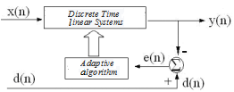
Figure 1. Principle of adaptive filter
The principle of adaptive filter is illustrated in Figure 1, where the discrete time linear system stands for an actual programmable filter, x(n) is the input of adaptive filter, y(n) is the output of the adaptive filter, d(n) is the desired output, and e(n) is the error inputted to the adaptive algorithm. Note that error is the difference between output and desired output.
The filter parameters of the adaptive filter can be characterized by the shock response h(n), which is affected by e(n). During the operation, the adaptive filter automatically adjusts the shock response such that the output gradually approaches the desired output.
Hence, the most significant difference between adaptive filter and ordinary filter lies in the fact that the adaptive filter can adjust its impulse response or filter parameters according to the external environment. After a while, the adaptive filter can achieve the optimal filtering effect.
The adaptive algorithm is critical to the performance of the adaptive filter. To track the changes in external environment, the adaptive algorithm must keep regulating filter parameters according to the preset criterion, considering the input, output and original values of the filter parameters. In this research, the LMS algorithm is selected as the adaptive algorithm [13].
3.1 Principle of LMS algorithm
The LMS algorithm is a linear adaptive filtering algorithm. The algorithm involves two operations, namely, filtering and adaptation. The goal is to minimize the mean square error of e(n)=d(n)-y(n) through parameter adjustment, and to modify weight accordingly. Given input and desired output, the LMS algorithm can achieve a small computing load without off-line calculation. There are many variants of the LMS algorithm. For example, the following LMS algorithm is coupled with the method of steepest descent [14].
$e(n)=d(n)-w(n-1) x(n)$ (1)
$W(n)=W(n-1)+2 \mu(n) e(n) X(n)$ (2)
where x(n) is the input of adaptive filter; d(n) is the desired output; e(n) is the error; w(n) is the weight; μ(n) is the step size. The filter parameters are adjusted by the adaptive algorithm in the light of error and input, aiming to minimize the error.
The convergence condition of the LMS algorithm is 0 <μ(n)< 1/λmax, where λmax is the maximum eigenvalue of the input autocorrelation matrix. The simplest way for parameter selection is to take the step size as a constant: μ(n) =μ (0 <μ <1/λmax). However, the fixed step size makes it impossible to achieve fast convergence, high tracking accuracy and small steady-state error at the same time. In other worse, the contradiction between convergence and stability will arise from the fixed step size. For instance, a high tracking accuracy helps to speed up the convergence, but increases the steady-state error; a low tracking accuracy improves steady-state performance, but slows down convergence.
3.2 LMS algorithm with variable step size
To solve the contradiction between convergence and stability, the LMS should adopt variable step size in different iterative processes. The basic ideas of the LMS algorithm with variable step size are as follows: in the initial phase, a large step size is needed to speed up convergence; then, the step size should be reduced with the growth in convergence speed, thus reducing the steady-state error.
In the existing LMS algorithms with variable step size, the step size is made proportional either to error or to the estimated cross-correlation of error and input. Practice shows that these algorithms can achieve fast convergence at a small tracking error, and effectively eliminate interferences. Besides, these algorithms are easy to implement with hardware, thanks to their small parameter size and computing load [15-16].
3.3 Improvement of LMS algorithm
The performance of LMS algorithm in adaptive filtering can be evaluated accurately by three technical indices: convergence speed, time-varying tracking accuracy and steady-state error. To solve the contradiction between these indices, the key lies in the design of the mapping relationship between step size and error.
Drawing on the abovementioned LMS algorithms with variable step size, this paper designs a new LMS algorithm with variable step size:
$W(n)=W(n-1)+2 \mu(n) e(n) X(n)$ (3)
$\mu(n)=\beta\left(1-\exp \left(-\alpha|e(n)|^{m}\right)\right.$ (4)
where α(>0) is the shape factor controlling the shape of function; β(>0) is the range factor controlling the value range of the function.
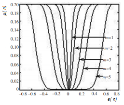
Figure 2. Relationship curves between step size and error
Figure 2 shows the relationship curves between step size and error at the range factor of 0.2, the shape factor of 10 and the exponential change factor (m) of 1, 2, 3, 4 and 6. It can be seen that, when m=1, the error oscillated about zero (i.e. the algorithm reached the steady state), and the step size fluctuated significantly rather than changing slowly; when m=2, the algorithm reached the steady state, the steps size changed very slowly; when m=3, the step size increased with the error in the initial phase of convergence and tracking, and changed slowly as the error approached zero (i.e. the algorithm was near the steady state); when m=4 and 6, the step size reached zero before the error approached zero (i.e. the algorithm was near the steady state), causing a high steady-state error, despite the gentle change at the bottom of the curve.
Considering the computing load, practical performance and other indices, the exponential change factor was set to 2. Then, the variable step length can be defined as:
$\mu(n)=\beta\left(1-\exp \left(-\alpha|e(n)|^{2}\right)\right.$ (5)
The LMS algorithm thus designed is very simple, and ensures that the step size change slowly after the error is stabilized. However, the algorithm is so sensitive to noise that it cannot achieve desired results on convergence speed, tracking accuracy and steady-state error at a low signal-to-noise ratio (SNR) [17-18].
To overcome this defect, the step size was no longer adjusted by the square of the error (e2(n)), but by the correlation between the current error and the error of a previous moment e(n-D), where D is a positive integer falling between the time-dependent radius of the input and that of the noise, after the error decreases to zero after a certain period. Since the autocorrelation of the noise drops to zero, the noise has much less impact on the step size, reducing the sensitivity of our algorithm to noise. The improved formula for variable step size can be expressed as:
$\mu(n)=1-\exp (-\alpha e(n) e(n-D))$ (6)
Thus, our algorithm now relies on the correlation value of the error e(n)e(n-D) to adjust the step size. This adjustment method fully considers convergence speed and steady-state error, and reduces the noise sensitivity of the algorithm with weak autocorrelation.
As mentioned before, the convergence condition of the LMS algorithm is 0 <μ(n)< 1/λmax, where λmax is the maximum eigenvalue of the input autocorrelation matrix. Thus, the range factor must be smaller than λmax: β< 1/λmax. Under this condition, the algorithm will eventually converge, and the step size will gradually decline and minimize after the convergence.
Figure 3. Relationship curves between step size and error of the improved LMS algorithm
Figure 3 presents the relationship curves between step size and error of the improved LMS algorithm at different shape factors and range factors. In the initial phase of convergence, the absolute value of the error was large, the step size was long and the algorithm converged rapidly. Once the algorithm reached the steady state, both the absolute value of the error and the step size were minimized.
It can be seen from Figure 3 that, when the initial error remained the same, the algorithm converged successfully with β< 1/λmax, and the convergence speed increased with the shape factor. Similarly, the convergence speed also increased with the range factor when the shape factor was constant. When the two factors were too large, however, the step size was very long at the convergence, despite the increase in convergence speed, resulting in a huge steady-state error.
Therefore, the shape factor and range factor should be selected to maximize the step size corresponding to the absolute value of the initial error, provided that the algorithm can still converge. In actual practice, the two factors should be optimized through experiments.
4.1 Advantages of step size setting
In our algorithm, the step size is no longer determined by the error in the current time, but by the correlation between the current error and the error in a previous moment e(n-D). This new method for step size setting has many advantages. For example, the autocorrelation error is usually close to the optimal value, making the adjusted step size suitable for application. Besides, the step size update will not be affected by irrelevant noise sequence. Due to the large initial adaptive error, the step size is long at the beginning. As the autocorrelation error approaches the optimal value (zero), the step size will stabilize at a small level. In the initial phase, the algorithm converges rapidly with the large step size; in the later phase, the tacking error can be minimized by the small step size. The step size becomes more accurate after considering the previous step sizes. Therefore, our algorithm can prevent the noise impacts more effectively than the traditional LMS algorithm [19-20].
4.2 Application in adaptive noise cancellation (ANC) system
In EPD systems, the received signals often contain many noises, which pushes up the bit error ratio. These signals should be denoised adaptively with the optimal filter. The optimal filter can be fixed or adaptive. A fixed filter needs to know the statistical properties of signals and noises, while the adaptive one requires no or little such knowledge.
The ANC system is responsible for enhancing the SNR through noise suppression or attenuation. The basic principle is to remove the noises from the noisy signals, in contrast to the desired output. The noise removal is known as noise cancellation, which relies on the correlation between the noisy signals and desired output. But the noises cannot be eliminated if the noisy signals are unrelated or weakly correlated. The residual noises will interfere with the filter and affect the adaptive algorithm.
Our algorithm provides a desirable way to solve this problem. The algorithm can distinguish between strong correlation noise and unrelated and weakly correlated noise. Here, the former is called additive noise signal n0 and the latter, the noise signal v.
Figure 4. The ANC mechanism of our algorithm
The ANC mechanism of our algorithm is illustrated in Figure 4, where n1 is the reference input. The main input contains the useful signal s to be extracted, the additive noise signal n0 and the noise signal v. The useful signal is not correlated with the noise signal, the additive noise signal or the reference input; the additive noise signal is related to the reference input, but not to the noise signal. The useful signal, the noise signal, the additive noise signal and the reference input are all zero mean signals. Hence, the output of the ANC system can be expressed as:
$e(n)=s(n)+n_{0}+v-y(n)$ (6)
Since useful signal is not correlated with the noise signal, the additive noise signal or the reference input, the mathematical expectation can be obtained by squaring both sides of equation (6):
$E\left(e^{2}\right)=E\left[(s+v)^{2}\right]+E\left[\left(n_{0}-y\right)^{2}\right]$ (7)
The term E[(s+v)2] is not affected by the adjustment of filter parameters to minimize the E(e2). Thus, the minimum output energy can be described as:
$E_{\min }\left(e^{2}\right)=E\left[(s+v)^{2}\right]+E_{\min }\left[\left(n_{0}-y\right)^{2}\right]$ (8)
The filter output y is the best estimate of the additive noise signal, for E[( s+v)2] is minimized at the minimal E(e2). As mentioned before, the error equals the difference between the output and desired output: e(n)=d(n)-y(n). In ideal conditions, the output equals the additive noise signal, and the error equals the useful signals. Hence, the error will infinitely approximate the useful signal.
If the application environment contains heavy noises, the noise signal v will have a great impact on the performance of the LMS algorithm. In this case, the traditional LMS algorithm cannot reach the optimal solution but oscillate about it. In our algorithm, the step size is adjusted by the correlation between the current error and the error of a previous moment e(n-D). In this way, our algorithm is no longer sensitive to noise while retaining the advantages of the traditional algorithm.
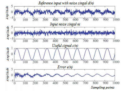
To verify its noise cancellation effect, our algorithm was applied to a simulation with an eight-stage finite impulse response (FIR) filter. The reference input to the adaptive filter was represented by a random number n1=randn(N,1), and the useful signal was set to s=sin(2*PI*10*t). Thus, the desired output d(n) is the sum of the useful signal and the reference input. The number of samples were set to 1,000 and the initial weight was set to zero.
Figure 5. Input and output of the filer
The simulation results are shown in Figures 5~6. The output was compared with the noisy signal and the useful signal, revealing that our algorithm completely removed the noises and restored the useful signal. Then, the discrete signals above were subjected to fast Fourier transform, producing their curves in the frequency domain (Figure 7). Obviously, our algorithm retained the useful signal and suppressed the frequency spectrum of the noises. In addition, our algorithm converged after fewer than 100 iterations, and controlled the steady-state error well. The simulation results show that our algorithm can converge rapidly with a good stability, and eliminate the noises in received signals.
Figure 6. Filtering effect in time domain
Figure 7. Filtering effect in frequency domain
This paper improves the traditional LMS algorithm with variable step size for adaptive filtering. Through the improvement, the step size is no longer adjusted by the square of the error (e2(n)), but by the correlation between the current error and the error of a previous moment e(n-D). In this way, the algorithm becomes less sensitive to the noise with weak autocorrelation, which is conducive to the adaptive filtering of noises. Our algorithm was verified through an ANC simulation. The results demonstrate the excellent steady-state performance and noise suppression effect of our algorithm.
Our algorithm solves the inherent contradiction of the LMS algorithm with fixed step size: the inability to achieve fast convergence, high tracking accuracy and small steady-state error at the same time. More importantly, our algorithm converges faster than the existing LMS algorithms with variable step size. The excellent performance is achieved with a simple structure and easy implementation steps. Therefore, our algorithm can be applied to many other fields of adaptive filtering, such as adaptive system identification and adaptive signal separation.
[1] Gao, Y., Xie, S.L. (2001). A variable step size LMS adaptive filtering algorithm and analysis. Chinese Journal of Electronics, 29(8): 1094-1097. https://doi.org/10.3321/j.issn:0372-2112.2001.08.023
[2] Zhang, Y.G., Chambers, J.A., Wang, W.W., Kendrick, P., Cox, T.J. (2007). A new variable step-size LMS algorithm with robustness to nonstationary noise. 2007 IEEE International Conference on Acoustics, Speech and Signal Processing, pp. 1349-1352. 10.1109/ICASSP.2007.367095
[3] Zhao, S., Man, Z., Khoo, S., Wu, H.R. (2008). Variable step-size LMS algorithm with a quotient form. Signal Processing, 8(1): 67-76. https://doi.org/10.1016/j.sigpro.2008.07.013
[4] Abdolee, R., Champagne, B., Sayed, A.H. (2013). Diffusion LMS strategies for parameter estimation over fading wireless channels. Proceedings of the IEEE International Conference on Communications (ICC), pp. 1926-1930 10.1109/ICC.2013.6654804
[5] Ren, Z.Z., Xu, J.C., Yan, Y.P. (2011). Improved variable step size LMS adaptive filtering algorithm and its performance analysis. Application Research of Computers, 28(3): 954-956. https://doi.org/10.3969/j.issn.1001-3695.2011.03.046
[6] Mayyas, K., Momani, F. (2011). An LMS adaptive algorithm with a new step-size control equation. Journal of the Franklin Institute, 348(4): 589-605. https://doi.org/10.1016/j.jfranklin.2011.01.003
[7] Mayyas, K. (2005). A new variable step size control method for the transform domain LMS adaptive algorithm. Circuits, Systems & Signal Processing, 24(6): 703-721. https://doi.org/10.1007/s00034-005-0705-7
[8] Zeng, X.X., Shao, Z.H., Lin, W.Z., Luo, H.B. (2018). Orientation holes positioning of printed board based on LS-Power spectrum density algorithm. Traitement du Signal, 35(3-4): 277-288. https://doi.org/10.3166/TS.35.277-288
[9] Zhu, Y.L., Xu, C.G., Xiao, D.G. (2019). Denoising ultrasonic echo signals with generalized s transform and singular value decomposition. Traitement du Signal, 36(2): 139-145. https://doi.org/10.18280/ts.360203
[10] Sristi, P., Lu, W.S., Antoniou, A. (2012). A new variable-step size LMS algorithm and its application in sub-band adaptive filtering for echo cancellation. IEEE International Symposium on Circuits and Systems, 1(2): 721-724. https://doi.org/10.1109/ISCAS.2001.921172
[11] Huang, H.C., Lee, J. (2012). A new variable step-size NLMS algorithm and its performance analysis. IEEE Transactions on Signal Processing, 60(4): 2055-2060. https://doi.org/10.1109/tsp.2011.2181505
[12] Chan, S.C., Chu, Y.J., Zhang, Z.G. (2013). A new variable regularized transform domain NLMS adaptive filtering algorithm-acoustic applications and performance analysis. IEEE Transactions on Audio, Speech and Language Processing, 21(4): 868-878. https://doi.org/10.1109/tasl.2012.2231074
[13] Li, W., Zhao, Z., Tang, J., He, F., Li, Y., Xiao, H. (2013). Performance analysis and optional design of the adaptive interference cancellation syestem. IEEE Transactions on Electromanetic Compatibility, 55(6): 1068-1075. https://doi.org/10.1109/temc.2013.2265803
[14] Dalers, C.J. (2014). A method of adaptation between steepest-descent and newton’s algorithm for multichannel active control of tonal noise and vibration. nternationnal Congress on Sound & Vibration, 19(3): 1-8. https://doi.org/10.13140/2.1.3647.2960
[15] Zheng Z., Liu, Z., Dong, Y. (2017). Steady-state and tracking analyses of improved proportionate affine projection algorithm. IEEE Transactions on Circuits and Systems II: Express Briefs, 65(11): 1793-1797. https://doi.org/10.1109/tcsii.2017.2767569
[16] Huang, B.Y., Xiao, Y.G., Ma, W.P., Wei, G. Sun, J.W. (2015). A simplified variable step size LMS algorithm for Fourier analysis and its statistical properties. Signal Processing, 117: 69-81. https://doi.org/10.1016/j.sigpro.2015.04.021
[17] Das, R.L., Chakraborty, M. (2015). On convergence of proportion- ate-type normalized least mean square algorithms. IEEE Transactions on Circuits and Systems II: Express Briefs, 62(5): 491-495. https://doi.org/10.1109/TCSII.2014.2386261
[18] Gui, G., Xu, L., Matsushita, S. (2015). Improved adaptive sparse channel estimation using mixed square fourth error criterion. Journal of the Franklin Institute, 352(10): 4579-4594. https://doi.org/10.1016/j.jfranklin.2015.07.006
[19] Chen, Y., Tian, J.P., Liu, Y.P. (2015). New variable step size LMS adaptive filtering algorithm. Electronic Measurement Technology, 38(4): 27-31. https://doi.org/10.19651/j.cnki.emt.2015.04.007
[20] Ni, J., Chen, J., Chen, X. (2016). Diffusion sign - error LMS algorithm: formulation and stochastic behavior analysis. Signal Processing, 128: 142-149. http://dx.doi.org/10.1016/j.sigpro.2016.03.022