Toualbia Asma*| Zegaoui Abdallah
OPEN ACCESS
A thermoelectric generator is silent and reliable, can be used to convert a temperature gradient to electricity based on the principles of Seebeck effect and vice versa. Very maximum power point tracker (MPPTs) are widely used in thermoelectric systems in order to extract the maximum available power for varying load and a given temperature difference. The perturbation and observation (P&O) algorithm are one of the most widely used due to ease of implementation. However, the operating point oscillates around the MPP that increase the loss of energy in the power of the TEM. Many improvements of the P&O algorithm have been proposed in order to reduce the oscillations. Therefore, in this paper, a P&O MPPT technique based on PI controller has been used for achieving the Maximum Power Point of a thermoelectric system. Performance of this technique is compared against the P&O based passivity control one through simulations.
thermoelectric generator, MPPT, DC/DC converter, passivity based control, Euler Lagrange
Thermoelectric energy is renewable source of energy, are able to convert the heat energy to electrical power. The thermoelectric generator consists of a number of thermocouples that are connected electrically in series to increase the voltage and thermally in parallel [1], as example, the HZ-20 module which it consists of 71 thermocouples [2, 3]. If a load is connected with the TEM HZ-20, a direct current flows and its power output of this device varies with temperature difference.
To extract maximum power from thermoelectric system, the Boost converter with MPPT controller is used. Many MPPT algorithms have been proposed in the literature [4]. The method of Perturb and observe (P&O) is the most commonly used because its ease and simple implantation. The main disadvantage of this algorithm that when the MPP is reached, the output power oscillates around the MPP [5]. Therefore, resulting in a power loss in the thermoelectric system.
In this paper, we propose an MPPT Perturb and observe algorithm based on a PI controller to achieve better TEM output performance. The main problem of using the PI controller is tuning its parameters to achieve optimum performance. However, the problems of stability get avoided in Perturb and observe based passivity control. The main purpose of this paper is to present a comparative analysis between the conventional Perturb and Observe (P&O) algorithm, the P&O method using a PI and the Perturb and observe based passivity for extracting the maximum power from the TEM system. The results show the Perturb and observe based passivity has much faster tracking time than the P&O method using a PI and the oscillation can be set to near zero.
This paper is organized as follows: section 1 presents the basic system configuration of the thermoelectric power generation system, operation characteristics, section 2 presents the theory of passivity (modeling of the Boost converter by Euler Lagrange) and a configuration of the algorithm perturb and observe based passivity approach (P&O/EL-PBC) MPPT. Section 3 discuss the simulation results with comparisons between a perturb and observe based passivity and a classical perturb and observe based PI in various situation, using MATLAB/SIMULINK tools and without it ending with the conclusions presented in section 4.
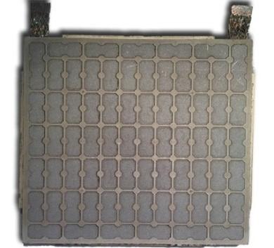
A typical thermoelectric generator power module is shown schematically in Figure1: Taking the HZ-20 module as an example, rated for 19W at ∆T=200 °C. It consists of 71 thermocouples connected electrically in series and thermally in parallel [1, 6].
Figure 1. HZ-20 thermoelectric module
The open-circuit thermoelectric potential VOC can be expressed as:
$V_{o c}=\alpha \Delta T$ (1)
where; α is the Seebeck coefficient.
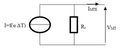
The Norton equivalent circuit of a practical TEM module is shown in Figure 2 [7].
Figure 2. Norton equivalent circuit for TEM
The output current IMTE of TEM module is given by:
$I_{M T E}=\frac{N_{S} \cdot \alpha_{p n} \cdot \Delta T-V_{M T E}}{N_{s} R_{i}}$ (2)
where, Ns number of TE thermocouples connected in series, and Ri electrical resistance of TEM.
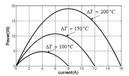
Figure 3 shows the output power generated as a function of the current for the HZ-20 TEG module. We can see that the output power increases with rising temperature difference.
Figure 3. P-I Characteristic of the module or different temperature gradients
The TEM will not automatically work at the MPP because it changes over the changes different temperature gradients. Maximum Power Point Tracking (MPPT) is used to track the MPP and makes TEM module work at the MPP all the time.
In any thermoelectric system, the output power can be increased by tracking the MPP of the TEM module by using a controller connected to a dc- dc converter (usually boost converter). By changing the duty cycle, the load impedance as seen by the source varies and matches at the point of the peak power with the source so as to transfer the maximum power. Various techniques have been proposed for tracking the MPP in the thermoelectric system; the most used algorithm is the Perturb and observe method [6]. It is based on the perturbation incrementing or decrementing the voltage and observing the result of this disturbance on the measured power. The algorithm oscillates around the peak point when the maximum power point is reached [8].
This oscillation around the MPP is one of the drawbacks of the method. For that, we propose an MPPT P&O algorithm based on a PI (Proportional Integral) controller [9]. The output signal u(t) delivered by the proportional and integral controller is proportional to both input signal V(t) and integral, as shown below:
$u(t)=K_{p} V_{i}(t)+K_{i} \int V_{i}(t)$ (3)
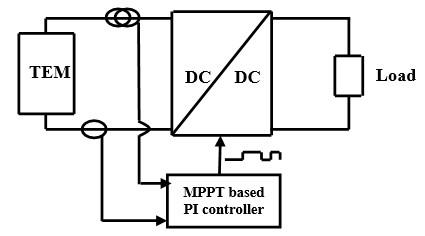
Figure 4 presents the block diagrams of the tracking system using the algorithm P&O based on a PI controller.
The MPPT block is used to generate the reference voltage (Vref) which is compared with the thermoelectric voltage (VTE) by the PI controller. The PI controller works towards minimizing the error between a both voltages by varies the duty cycle of the boost converter. The simulation results for different conditions are discussed in the last part.
Figure 4. Block diagrams of the algorithm P&O using PI controller
One disadvantage of the P&O based PI is the stability and dynamic performances are impossible [5]. In the next section, a comparative study of the Perturb and Observe (P&O) based PI algorithm, and the Perturb and Observe based passivity is given. A simulation to verify the effectiveness of the algorithm is described next, and the results are complemented by a comprehensive discussion.
Perturb and Observe based passivity use to have a faster controller response and to increase system stability once reached the MPP. This technique demonstrates its effectiveness and makes it among the best control for the tracking MPP. In this article a Lagrangian dynamics is presented.
5.1 The basic principles of Lagrangian
The Lagrangian of the system is represented by the differential equation as follows [10-11]:
$\frac{d}{d t} \frac{\partial L(q, \dot{q})}{\partial \dot{q}}-\frac{\partial L(q \dot{q})}{\partial q}=-\frac{\partial F(\dot{q})}{\partial \dot{q}}+Q$ (4)
where:
L: The Lagrangian of the system, represented as the magnetic co-energy of the inductive elements and the electric field energy of the capacitive elements:
$L(q, \dot{q})=T(\dot{q}, q)-V(q)$ (5)
T: is kinetic energy.
V: is potential energy.
F: the Rayleigh dissipation function is given by:
$F_{q}=\frac{1}{2} \dot{q}^{T} R \dot{q}$ (6)
Q: exogenous inputs to the system.
5.2 Modeling of Boost converter by Lagrangian
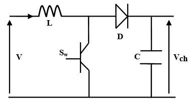
Figure 5 shows basic circuit of a DC-DC boost converter circuit. The DC-DC boost converter will boost up the output voltage to be higher than input voltage [7].
Figure 5. Boost converter
The subsystem’s Euler-Lagrange model is established as follows:
$\left\{\begin{array}{c}{T_{\mu}(\dot{q})=\frac{1}{2} L q_{L}^{2}} \\ {V_{\mu}(q)=\frac{1}{2 C} q_{C}^{2}} \\ {F_{\mu}(\dot{q})=\frac{1}{2} R_{c h}\left((1-\mu) \dot{q}_{L}-\dot{q}_{C}\right)^{2}} \\ {Q_{\mu}=\left(\begin{array}{c}{V} \\ {0}\end{array}\right)}\end{array}\right.$ (7)
where qL and qC are the quantity of charge in the inductance and the output capacitance respectively. Moreover, the switch position takes the value 0 or 1. Now, Lagrangian can be formulated as:
$L_{\mu}(q, \dot{q})=T_{\mu}(\dot{q})-V_{\mu}(q)=\frac{1}{2}\left(L \dot{q}_{L}^{2}-\frac{q_{C}^{2}}{C}\right)$(8)
Then, by replacing (7) and (8) in (4) it yields to:
$\left(\begin{array}{cc}{L} & {0} \\ {0} & {C}\end{array}\right) \dot{x}=\left(\left(\begin{array}{cc}{0} & {-(1-\mu)} \\ {1-\mu} & {0}\end{array}\right)-\left(\begin{array}{cc}{0} & {0} \\ {0} & {\frac{1}{R_{c h}}}\end{array}\right))x+\left(\begin{array}{c}{V} \\ {0}\end{array}\right)\right.$ (9)
That is, the input current defined as $x_{1}=\dot{q}_{L}$ and the output voltage capacitor is represented as $x_{2}=q_{c} / C$. Thus, the model of our system (equation 9) is described in Lagrangian form;
$M \dot{x}+(1-\mu) J x+R x=E$ (10)
where M the diagonal matrix, and where J=-JTantisymmetric and its element are given by (-1, 0, 1). Then the vector E=[V 0] represents the exogenous inputs.
$M=\left(\begin{array}{cc}{L} & {0} \\ {0} & {C}\end{array}\right) \quad J=\left(\begin{array}{cc}{0} & {1} \\ {-1} & {0}\end{array}\right) R=\left(\begin{array}{cc}{0} & {0} \\ {0} & {\frac{1}{R_{c h}}}\end{array}\right)$
Thus, we introduce the damping injection function in the system to ensure the asymptotic stability.
The damping injection function consists in modifying the Rayleigh dissipation function as follow:
$R=R_{d}-R_{B}$ (11)
where:
Rd: the desired dissipation.
RB: the injected damping matrix.
The injected damping matrix can be described through the following equation:
$R_{B}=\left(\begin{array}{cc}{R_{1}} & {0} \\ {0} & {0}\end{array}\right)$ (12)
We consider that a storage function of the system can be chosen according to the form:
$H(x)=\frac{1}{2} x^{T} M x$ (13)
So, we can propose as a desired storage function:
$H_{d}(x)=\frac{1}{2} \widetilde{x}^{T} M \widetilde{x}$(14)
where:
$\breve{\mathcal{X}}$ ; Then, xd desired value of x.
If we replace the error dynamics $\breve{\mathcal{X}}$ in the system equation (10), we find:
$M \dot{\tilde{x}}+(1-\mu) J \tilde{x}+R \tilde{x}=$
$E-M \dot{x}_{d}-(1-\mu) J x_{d}-R x_{d}=\Phi$ (15)
We ensure the stabilization of our system, if we set the Φ=0.
$M \dot{\tilde{x}}+(1-\mu) J \widetilde{x}+R \widetilde{x}=0$ (16)
The error behavior is asymptotically stable to zero; it means that is independently of µ.
In order to satisfy (16), one must demand:
$M \dot{x}_{d}+(1-\mu) J x_{d}+R x_{d}-R_{1 B} \widetilde{x}=E$ (17)
Finally the scalar form:
$\left\{\begin{array}{c}{L \dot{x}_{1 d}+(1-\mu) x_{2 d}-R_{1}\left(x_{1}-x_{1 d}\right)=V} \\ {C \dot{x}_{2 d}-(1-\mu) x_{1}+\frac{1}{R_{c h}} x_{2 d}=0}\end{array}\right.$ (18)
Then, the solving of equation (18) results:
$\mu=1-\frac{1}{V_{d}}\left(V+R_{1}\left(I_{L}-\frac{V_{d}^{2}}{V \cdot R_{c h}}\right)\right)$ (19)
where:
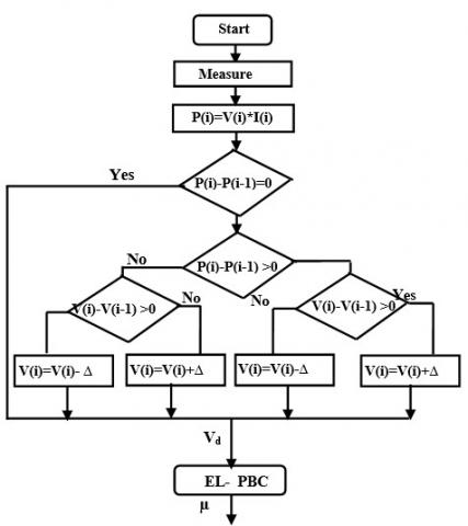
Vd: is the output MPPT P&O voltage delivered to the passivity bloc control system.
Figure 6. P&O/PBC MPPT algorithm
In this section, the responses of the P&O MPPT, the P&O based a PI controller and the P&O MPPT based passivity are presented and analyzed. The TE system was simulated in MATLAB/SIMULINK. The TEM module (HZ-20) which is taken as the reference TEM module for the simulation, the manufacturer’s data sheet details for this module are given in Table 1.
Table 1. The TEM module parameters [2]
|
Property |
value |
|
Width and length |
7.5cm |
|
Design hot side temperature |
230°C |
|
Design cold side temperature |
30°C |
|
Maximum temperature |
250°C |
|
Power and matched load |
19watts |
|
Load voltage |
2.38volts |
|
Internal resistance |
0.2981ohm |
The results of the output power, voltage and current of the TME for different temperature gradients ∇T=200℃ are depicted in Figure 7, Figure 8 and Figure 9.
Figure 7. TEM output power at ∇T=200℃
Figure 8. TEM output power at ∇T=200℃
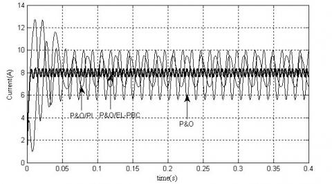
Figure 9. TEM output current at ∇T=200℃
From the simulation results, we can observe that the P&O/EL-PBC shows the best performance in both the total power (less steady state oscillations) and the response time (faster settling time) against the P&O and the P&O/PI algorithms, resulting in higher energy produced by the TEM module. the Figure 7 and Figure 8 show the output waveforms of the voltage and current, the results illustrates that the P&O/EL-PBC MPPT reaches faster to the optimal voltage and current with less oscillations compared to the both MPPT.
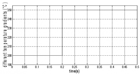
Figure10. Difference temperature gradients of the TEM
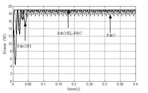
The Figures (11), (12) and (13) show the simulations results concerning the power, voltage and current of the TME module during a change in different temperature gradients from ∇T=200℃ to ∇T=250℃ at t=0.2sec.
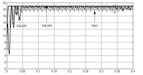
As shown by Figure11, it can be noticed that the P&O/EL-PBC can track the maximum power at 0.005s compared to the P&O MPPT and P&O/PI tracked the MPP at the 0.06s and 0.05s respectively. Besides, the TEM power is more stable than the P&O/EL-PBC controller. On the other hand, at the t=0.2s, we apply a sudden change in the different temperature gradients, it can be observed that the P&O/EL-PBC can reduced the power loss compared the P&O/PI.
Figure 11. The power of the TEM
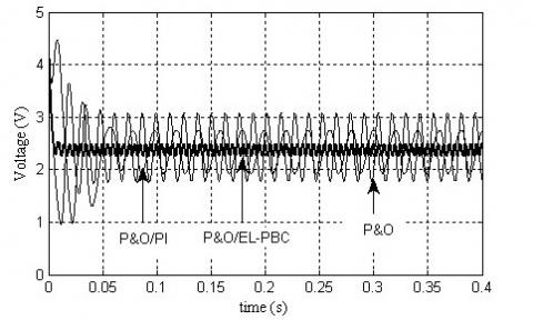
Figure 12. The voltage of the TEM
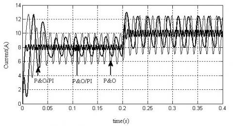
Figure 13. The current of the TEM
From the observation of Figure 12 and Figure 13, it can see that the operating voltage and current of TEM system controlled by the P&O MPPT and P&O/PI controller are fluctuated around the MPP. However, the P&O/EL-PBC MPPT have ability to reduce the perturbed voltage and current.
The comparison of the power efficiencies of the different MPPT controllers is shown in Table 2.
Table 2. The performances of the three MPPT methods
|
MPPT methods |
|
Efficiency (%) |
|
|
different temperature gradients constant |
Different temperature is variable |
|
P&O |
91.06 |
96.32 |
|
P&O/PI |
95.95 |
97.64 |
|
P&O/EL-PBC |
99.79 |
99.79 |
6.3 Simulation results for sudden changes in the load
In this section, we study the behavior of the system thermoelectric to the sudden change of the load. The load resistance is changed from R=3Ω to R=3.5Ω at t=0.21s.
Figure 14. The power of the TEM
In the Figure 14, we can see that the P&O/EL-PBC has good performance compared with a PI controller, it performs a small power loss at time t=0.34s. The efficiency of this algorithm is 99.99 % respectively.
This paper presents the comparison of P&O MPPT, P&O besed PI and P&O/EL-PBC in relation to their performance. The results indicate that P&O/PI method has low efficiency because of its lack of speed in tracking the MPPT. But, the P&O/EL-PBC method shows the effectiveness of the last to eliminate the oscillations and achieve less response time successfully.
This article is dedicated to late Mohammed Bederrar associated to this work and who recently left us. A.A.B. thanks M.Tadjine for their helps in some specific parts of this project.
|
Symbol |
Significance |
|
P&O |
Perturb and Observe, |
|
MPPT |
Maximum Power Point Tracking, |
|
PBC |
Passivity based control, |
|
P&O/PBC |
Perturb and Observe based passivity, |
|
TEM |
Thermoelectric Module, |
|
EL-PBC |
the Euler Lagrange passivity based control, |
|
Voc |
The open-circuit thermoelectric potential, |
|
α |
the Seebeck coefficient, |
|
∆T |
is the temperature difference across the two junctions, |
|
ρ |
the electrical resistivity, |
|
K |
the thermal conductivity, |
|
Vg |
the generated Seebeck voltage, |
|
V |
the voltage of TEM, |
|
Rg |
total electrical resistance of TEM, |
|
Vm |
The maximum voltage, |
|
P |
The power of the load, |
|
Vch |
Voltage of the load, |
|
L |
The Lagrangian of the system, |
|
T |
the electric field energy, |
|
D |
the Rayleigh dissipation, |
|
Fq |
exogenous inputs to the system, |
|
qL |
the electrical charge on the inductor, |
|
qC |
the electrical charge on the capacitor, |
|
μ |
the duty cycle of the converter, |
|
Rb |
The injected damping matrix, |
|
Rd |
the desired error dissipation, |
|
$\widetilde{x}$ |
the error state vector, |
|
X1d |
the desired inductor current, |
|
X2d |
the output MPPT P&O voltage delivered, |
|
H(x) |
the energy storage function, |
|
Hd(x) |
the energy storage function desired |
[1] Tang, Z.B., Deng, Y.D., Su, C.Q., Shuai, W.W., Xie, C.J. (2015). A research on thermoelectric generator's electrical performance under temperature mismatch conditions for automotive waste heat recovery system. Case Studies in Thermal Engineering, 5: 143-150. https://doi.org/10.1016/j.csite.2015.03.006
[2] Tsai, H.L., L, J.M. (2009). Model building and simulation of thermoelectric module using Matlab/Simulink. Journal of Electronic Materials, 39(9): 2105-2111. https://doi.org/10.1007/s11664-009-0994-x
[3] Gao, H.B., Huang, G.H., Li, H.J., Qu, Z.G., Zhang, Y.J. (2016). Development of stove-powered thermoelectric generators: A review. Applied Thermal Engineering, 9: 297-310. https://doi.org/10.1016/j.applthermaleng.2015.11.032
[4] Ludek, J., Zdenek, H. (2015). Power management electronics for thermoelectric energy harvesting systems. International Journal Engineering, 13(1): 183-186.
[5] Paraskevas, A., Koutroulis, E. (2016). A simple maximum power point tracker for thermoelectric generators, Energy Conversion and Management, 108: 355-365. https://doi.org/10.1016/j.enconman.2015.11.027
[6] Singh, M., Bhukesh, S.K., Vaishnava, R. (2015). Modeling and simulation of solar thermoelectric generator. IOSR Journal of Electrical and Electronics Engineering, 10(3): 71-76. 10.9790/1676-10337176
[7] Toualbia, A., Tadjine, M. (2017). Perturb and observe maximum power point tracking based passivity approach for thermoelectric generator. The Mediterranean Journal of Measurement and Control, 13(1): 355-365.
[8] Abouda, S., Nollet, F., Essounbouli, N., Chaari, A., Koubaa, Y. (2013). Design, simulation and voltage control of standalone photovoltaic system based MPPT: application to a pumping system. International Journal of Renewable Energy Research, 3(3): 539-549.
[9] Sreekala, P. Ramkumar, A. (2017). Performance analysis of thermoelectric generator with different controllers. Technical Research Organization India, 4(11): 13-16. https://doi.org/10.3390/e17117387
[10] Belabbes, B., Lousdad, A., Meroufel, A., Larbaoui, A. (2013). Simulation and modelling of passivity based control of PMSM under controlled voltage. Journal of Electrical Engineering, 64(5): 298-304. https://doi.org/10.2478/jee-2013-0043
[11] Tofighi, A., Kalantar, M. (2013). Interconnection and damping assignment and Euler-Lagrange passivity-based control of photovoltaic/battery hybrid power source for stand-alone applications. Journal of Zhejiang University- Science (Computers & Electronics), 12(9): 774-786. https://doi.org/10.1631/jzus.c1000368