VSSN Gopala Krishna Pendyala* | Hemantha Kumar Kalluri | Venkateswara C. Rao
OPEN ACCESS
The purpose of this study is to investigate the best suitable pan sharpening method for CARTOSAT-2E satellite launched by ISRO (Indian Space Research Organisation). This satellite provides high resolution images that are being used for many urban applications such as mapping, feature extraction, facility management etc. The synthesized image using pan sharpening method enables users to take the combined advantage of the best available spatial and spectral resolutions. In this paper, various pan sharpening methods based on component substitution (CS) and Multi Resolution Analysis (MRA) are applied on the CARTOSAT-2E images and the resultant images are tested for their qualitative and quantitative performance. Qualitative analysis is carried out based on image blur and spectral distortion and quantitative evaluation is performed using image metrics by comparing the synthesized image with the original image. The results show that the High-Pass Filter (HPF) method offers the good spectral fidelity. However, due to its inherent stair-casing effect in the resultant image; modified-IHS followed by PRACS method is found to be preferable for automatic urban feature extraction from CARTOSAT-2E images.
component substitution, high resolution satellite image, multi resolution analysis, pan sharpening, urban feature extraction
High resolution Remote Sensing satellite images provide/have finer details of the earth surface that helps in better management of natural resources and disasters. CARTOSAT-2E satellite is equipped with panchromatic (PAN) and multispectral (MS) sensors. The panchromatic sensor provides gray scale images with high spatial resolution and the multispectral sensor provides multi-band images with color data (multi spectral) having low spatial resolution compared to panchromatic image [1]. However, acquisition of both high spatial and high spectral resolution in a single image is not possible due to non-availability of sensor technology and system design tradeoffs.
High resolution satellite sensors paved the way for the development of image fusion techniques. The fusion of the multispectral data with the panchromatic satellite images offers the advantages of high spatial and spectral resolution simultaneously [2, 3]. Pan-sharpening is a fusion operation capable of integrating different images from a single sensor to produce synthesized images having maximum enhancement of the spatial details at minimum spectral distortion [4]. The general idea behind pan sharpening is to preserve the spectral values of the multispectral image and to improve the spatial resolution. The resultant fused images can be used for remote sensing applications as an input data to derive useful information, by applying enhanced image processing techniques, segmentation, classification and object detection [2].
High resolution satellite images have a typical spatial resolution of less than 1.0 m for panchromatic band and 3 to 4 times that for multispectral data. Various HR satellites such as, IKONOS, QuickBird, GeoEye and Worldview are offering data in the form of simultaneous acquisition (coregistered) of the single band PAN imagery and 4 to 8 band MS imagery [3, 5, 6].
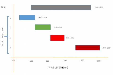
Figure 1. Spectral bands of CARTOSAT-2E
The CARTOSAT-2E satellite of Indian Space Research Organization (ISRO) provides images in a single PAN and four MS bands at a spatial resolution of 0.60 m and 1.6 m simultaneously at 11 bit radiometric resolution [7]. The PAN image can take panchromatic (black and white) in a selected portion of the visible and near-infrared spectrum (0.50–0.85 µm). The 4-channel MS records data of spectral resolutions 0.43 - 0.52 µm, 0.52 - 0.61 µm, 0.61 - 0.69 µm, 0.76 - 0.90 µm in 4 separate bands as shown in Figure 1. This study is carried out on urban area of CARTOSAT-2E dataset to find the suitable pan sharpening method for urban feature extraction and large-scale mapping applications.
The remainder of this paper is organized as follows: In section two review of various pan sharpening approaches used for this study are presented; section three describes evaluation methods and metrics; section four describes the data sets, and experiments; section five presents the results and analysis; and finally, conclusions are drawn in Section six.
Many proven methods are available in which the spatial details of the panchromatic image of better resolution are induced into the multispectral image of lower spatial resolution [4]. The fusion operations use many computational techniques such as filtering, regression, decomposition, numerical computing, orthogonal transformation, wavelet transformation, and pyramid decomposition. Two main categories based on spatial and spectral theme (i) Component Substitution (CS) techniques and the Multi-Resolution Analysis (MRA) respectively are used. Other methods based on sensor response [8], Laplacian and Curvlet transform [9] and hybrid methods [10] are also implemented.
2.1 Component substitution
CS method projects the MS image into another dimensional space, which separates spatial and spectral components. Subsequently, the spatial component will be replaced with the PAN image or some of its information. Spectral distortion will be less in the fusion if the correlation between the PAN image and the replaced component has similar variations [11]. The statistics of both images are correlated by using a procedure such as histogram-matching before replacing the PAN image to match spectrally with that component. Finally, by applying the inverse spectral transformation, the fusion process is completed.
Component Substitution method is a global approach operating in the same way on the whole image and produce high spatial fidelity but poor spectral fidelity as they do not account for local dissimilarities between PAN and MS images. Brief description of the CS based methods used for this study are provided below with the detailed explanation in the references [5, 6, 9, 12-14].
A general formula for CS method follows the following equation:
$\dddot{M S}_{l}=\overline{M S}_{l}+g_{i}\left(P-I_{L}\right), \quad i=1, \ldots N$ (1)
where, $\dddot{M S}_{l}$ represents the fused image, and $\overline{M S}_{l}$ represents the up sampled MS image, P is the high resolution PAN image, i is the $i^{t h}$ spectral band and $g_{i}$ is the injection gain of the $i^{t h}$ band [13, 14]. $I_{L}$ is the synthetic intensity image derived from MS image, defined by:
$I_{L}=w_{i} \sum_{i=1}^{N} \widetilde{M S_{l}}$ (2)
where, wi is the weight of the ith band and the number of bands in MS image is indicated by N.
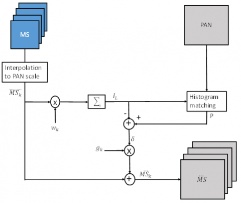
Figure 2. CS pan sharpening procedure [13, 14]
The schematic diagram is shown in Figure 2 and the pan sharpening techniques used for this study are described below:
2.1.1 Intensity Hue Saturation (IHS)
The MS image is first transformed into IHS colour space by dividing it to intensity (I), hue (H) and saturation (S) components. The PAN image and the I component are scaled to have same mean and variance and then the I component is replaced with the PAN image. As a final step, the inverse transform on the IHS is applied to get the fused image [2, 5, 11].
$\dddot{M S}_{k}=\overline{M S_{k}}+\left(\sum_{i=1}^{N} w_{i}\right)^{-1}\left(P-I_{L}\right), \quad k=1, \ldots N$ (3)
where, $I_{L}$ follows from Eq. (2) and the weight factor $w_{i}$ for all bands is equal to 1/N.
2.1.2 Modified IHS
As the name suggests, it is a modified version of IHS method described previously. It works best where there is significant overlap of the wavelengths of the merging images as the weights are assessed based on the spectral overlap between each MS band and PAN image. Running multiple passes of the algorithm merge function enables images with more than three bands to be merged [13].
2.1.3 Brovey Transform (BT)
This transformation represents a multiplicative sharpening [2, 5]. Uses spatial modulation of spectral pixels following Eq. (1) with weight function is 1/N and injection gain as following:
$g_{k}=\frac{\overline{M S_{k}}}{I_{L}} \quad k=1, \ldots . N$ (4)
2.1.4 Principle Component Analysis (PCA)
PCA of the MS image is achieved by transforming MS image to feature space through multidimensional rotation of the spectral bands. The first principal component (PCA1) has the highest variance and carries the maximum spatial de-correlations observed in MS image. This PCA1 is replaced by PAN image and the fused MS image is obtained by the inverse transformation [2, 6, 10, 12].
2.1.5 Gram-Schmidt Fusion (GS)
Gram-Schmidt transformation is a generalization of PCA, in which the PCA1 is substituted with the simulated the PAN band from the lower spatial resolution spectral bands. The simulated PAN band is first adjusted and matched for the statistics with the higher spatial resolution PAN [2, 6, 10-12]. This fusion process follows Eq. (1) with weight function 1/N and injection gain.
$g_{k}=\frac{\operatorname{cov}\left(\overline{M S_{k}}, I_{L}\right)}{\operatorname{var}\left(I_{L}\right)} \quad k=1, \ldots N$ (5)
in which, $\operatorname{cov}\left(\overline{M S_{k}}, I_{L}\right)$ is the covariance between two images $\overline{M S_{k}}$ and $I_{L}$, and $\operatorname{var}\left(I_{L}\right)$) is the variance of $I_{L}$.
2.1.6 Partial Replacement Adaptive Component Substitution (PRACS)
The PRACS generates high-/low-resolution synthetic component images by partial replacement method and uses a statistical ratio-based high-frequency injection [6, 9]. The algorithm utilizes the weighted sum of PAN and of the $k^{t h}$ MS band, to calculate the sharpened $k^{t h}$ band as per Eq. (1), where the weights $w_{k}$ are obtained through the linear regression of MS and using the correlation coefficient between PAN and MS bands.
2.2 Multi-Resolution Analysis (MRA)
MRA methods are intended to retain the spectral information of MS image and inject further information of high spatial resolution PAN image. Spatial filter is used to extract the spatial information at different scale levels from the PAN image and this information is used to perform Multi resolution analysis. The main advantage of these methods is the spectral coherency.
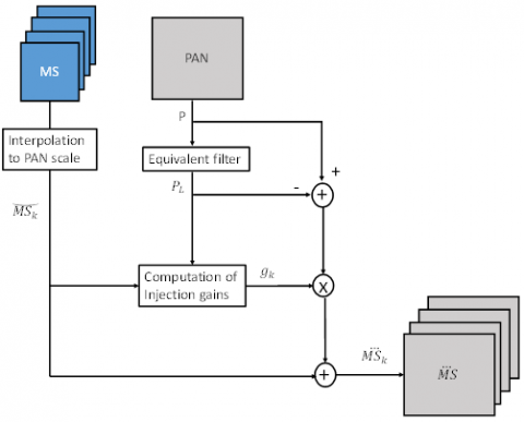
In this method the contribution of the PAN image to the fused product is achieved by calculating the difference between P and the low pass version PL [13]. The formula for MRA based methods can be represented by the Eq. (6) and its schematic diagram is shown in Figure 3.
Figure 3. MRA pan sharpening procedure [13, 14]
$\dddot{M S}_{k}=\overline{M S_{k}}+g_{k}\left(P-P_{L}\right), \quad k=1, \ldots N$ (6)
The higher spatial details to be injected into MS image are provided by P-PL by where PL is the modified component of the PAN band. The approach in obtaining PL varies for each the method.
The injection scheme is defined based on the gain gk. For $g_{k}=1$ for $k=1, \ldots N$, it is referred as additive injection scheme and for $g_{k}=\frac{\overline{M S_{k}}}{P_{L}}$ for $k=1, \ldots N$ it is referred as multiplicative injection scheme [12].
Some of the MRA based methods used for this study are briefly explained below with the detailed explanations are provided in the references [5, 6, 12-14].
2.2.1 High Pass Filter (HPF)
The process involves modification of Eq. (6) consisting of convolution using a low pass box filter (having uniform weights) $h_{L P}$ to the PAN image P for obtaining PL with additive injection gain [6, 11] shown below:
$\dddot{M S}_{k}=\overline{M S_{k}}+g_{k}\left(P-P * h_{L P}\right) \quad k=1, \ldots N$ (7)
2.2.2 Smoothing Filter-based Intensity Modulation (SFIM)
The SFIM algorithm is a variant of HPF as per Eq. (7) by employing the high pass modulation (HPM) injection methodology [10, 12, 15] thus having a gain factor as $\frac{\overline{M S_{k}}}{P_{L}}$ for $k=1, \ldots N$.
2.2.3 A tróus Wavelet Transformation (ATWT)
The low frequency component of PAN image from the PAN image to n wavelet planes (n = 2 or 3) generated by the “à trous” wavelet and adding the wavelet planes (i.e., spatial details) to each of the MS spectral bands [6-9, 11]. The low pass filter kernel for the A tróus non-orthogonal undecimated wavelet transform is defined by [8, 16]:
$A=\frac{1}{256}\left[\begin{array}{ccccc}1 & 4 & 6 & 4 & 1 \\ 4 & 16 & 24 & 16 & 4 \\ 6 & 24 & 36 & 24 & 6 \\ 4 & 16 & 24 & 16 & 4 \\ 1 & 4 & 6 & 4 & 1\end{array}\right]$ (8)
2.2.4 Proportional AWL (AWLP)
Both PAN and Intensity components are decomposed into wavelet planes and the spatial details of PAN image are adaptively injected based upon the proportions between each MS band and their summation in order to obtain a merged intensity component [6-9, 11, 13]. The injection gain is defined as:
$g_{k}=\frac{\overline{M S_{k}}}{\frac{1}{N} \sum_{I=1}^{N} \overline{M S_{k}}} \quad k=1, \ldots N$ (9)
The objective of the pan sharpening is to synthesize an image that could have been acquired with an original sensor of single high resolution spatial and spectral sensor. As stated previously, this could not be directly achieved either due to practical limitations of the technology or system design constraints.
Once, the pan sharpened image is produced, different quality measurements are applied to analyze the spatial and spectral fidelity of the pan sharpened image. Quality analysis is performed using qualitative and quantitative measurements.
3.1 Qualitative analysis
Qualitative analysis is carried out by visually inspecting for artifacts such as blur and spectral distortion [17] and comparing the results.
3.1.1 Blur
Blur occurs near transition areas and edges. It is also observed in the image due to in-sufficient spatial information of small features compared to sensor resolution and spectral mixing of smaller objects [17].
3.1.2 Spectral distortion
Occurs when the pan sharpening method try to include the spectral information to the improved spatial content compared to the reference.
3.2 Quantitative analysis
This analysis is carried out by numerical methods to compare fused image to the original PAN/MS images. There are different parameters that can be derived depending on the non-availability/ availability of reference images. The metrics used for evaluation of the images synthesized are described briefly in this section and detailed explanations are provided in the references [1, 10, 12, 13, 18, 19].
3.2.1 Correlation Coefficient (CC)
The CC is global parameter calculated for the entire image by comparing the original image A, and the fused image B. It is defined as:
$C C(A, B)=\frac{\sum_{m n}\left(A_{m n}-\bar{A}\right)\left(B_{m n}-\bar{B}\right)}{\sqrt{\left(\sum_{m n}\left(A_{m n}-\bar{A}\right)^{2}\left(B_{m n}-\bar{B}\right)^{2}\right)}}$ (10)
where, $\bar{A}$ and $\bar{B}$ stand for the mean values of the respective images [2, 10, 12, 18, 19]. A CC value of +1 indicates high correlation among the images.
3.2.2 Root Mean Square error (RMSE)
It measures the changes in the radiance of the pixel values of the input MS image A and pansharpened image F. The formula for RMSE is:
$R M S E=\sqrt{\frac{\sum_{x} \sum_{i}\left(A_{i}(x)-F_{i}(x)\right)^{2}}{M \times N \times d}}$ (11)
where, x is the pixel, d is the number of bands and i is the band number. M and N are the number of rows and columns [2, 10, 12, 18, 19]. The value should be close to zero.
3.2.3 Peak Signal to Noise Ratio (PSNR)
PSNR can be calculated for comparing both spatial and spectral fidelity. It is computed as:
$P S N R=10 \times \log _{10}\left(\frac{L^{2}}{R M S E^{2}}\right) \mathrm{Ffi}$ (12)
L is the peak value in a given image [18, 19]. Higher PSNR represents better response.
3.2.4 ERGAS (Erreur Relative Globale Adimensionnelle de Synthese)
It is based on calculating mean shifting and dynamic range and the formula for ERGAS is given by:
$E R G A S=100 \frac{h}{l} \sqrt{\frac{1}{N} \sum_{i=1}^{N}\left(\frac{R M S E(i)}{\mu(i)}\right)^{2}}$ (13)
The ratio of pixel sizes between PAN and MS images is $\frac{h}{l}$, the mean of the $i^{t h}$ band is $\mu(i)$ for N bands. ERGAS is global quality index which is dimensionless and lower values indicate higher spectral quality of the fused image [10, 11].
3.2.5 Spectral Angle Mapper (SAM)
The result of the comparison is reported as the angular difference (in radians) between the two spectra. The formula for SAM at a specific pixel is given by:
$\cos \alpha=\frac{\sum_{i=1}^{N} A_{i} B_{i}}{\sqrt{\sum_{i=1}^{N} A_{i} A_{i}} \sqrt{\sum_{i=1}^{N} B_{i} B_{i}}}$ (14)
For N number of bands, $\alpha$ is the spectral angle at a pixel having for A and B spectral vectors with the same wavelength from the MS and pan sharpened image, respectively. Average of all $\alpha$ values provide SAM for the entire image [10-12, 17, 18]. Small angles indicate high similarity.
3.2.6 Structural Similarity Index Measure (SSIM)
SSIM index is the averaged correlations for entire image for structural, luminance and contrast between MS and pan sharpened images.
$\operatorname{SSIM}(x, y)=\frac{\left(2 \mu_{x} \mu_{y}+C_{1}\right)\left(2 \sigma_{x y}+C_{2}\right)}{\left(\mu_{x}^{2}+\mu_{y}^{2}+C_{1}\right)\left(\sigma_{x}^{2}+\sigma_{y}^{2}+C_{2}\right)}$ (15)
where, μx and μy represent the means, σ x and σ y are the sample variances, and σ xy is the sample correlation coefficient between x in MS and corresponding y in pan sharpened image [2, 10, 18, 19]. Its value should be close to one.
3.2.7 Universal Image Quality Index (UIQI)
Distortion is estimated as a combination of loss of correlation and distortions in luminance, and contrast.
$Q=\frac{4 \sigma_{x y} \overline{x y}}{\left(\sigma_{x}^{2}+\sigma_{y}^{2}\right)\left[(\bar{x})^{2}+(\bar{y})^{2}\right]}$ (16)
x and y the original MS and fused image vectors $\bar{x}, \bar{y}$ are the mean values and $\sigma_{x}^{2}$ and $\sigma_{y}^{2}$ represent the RMS error [8, 18].
The value is estimated separately for each band and average is obtained for all bands. The value should approach close to 1 for better quality.
3.2.8 Q4
The Q4 index is a generalization of the Q index and defined by:
$Q 4=\frac{\left|\sigma_{z 1, z_{2}}\right|}{\sigma_{z_{1}} \sigma_{z_{2}}} \times \frac{2 \overline{\left|\overline{z_{1}}\right|}\left|\overline{z_{2}}\right|}{|\bar{z}|_{1}^{2}+\left|\overline{z_{2}}\right|^{2}} \times \frac{2 \sigma_{z_{1}} \sigma_{z_{2}}}{\sigma_{z_{1}}^{2}+\sigma_{z_{2}}^{2}}$ (17)
where, z1 is the radiance vector of MS image and z2 be the radiance vector of pan sharpended image which comprises of all the band radiance information. The higher the quality of the image is, the higher is the metric Q4 [11, 18, 20].
3.3 Evaluation methodology of the synthesized images
The planimetry accuracy of the fusioned image can be evaluated by standard method as recommended in reference [21]. A formal approach for quality assessment of the generated synthetic images was proposed by Wald et al. [22] and it is being widely accepted method by researchers. It is to be noted that, any pan sharpened image, should be identical to its original image when it is degraded to its original resolution and also should be identical to the image that will be produced by the sensor having that higher resolution. Hence, it is required to degrade or scale down the pan sharpened images to the original MS scale before testing the image quality further.
4.1 Dataset
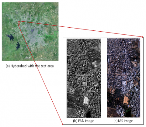
Study area covering an urban area of 2 km² of Hyderabad was subset from the full scene of CARTOSAT-2E acquired on January 1, 2018 (MS and PAN both) for investigation purpose.
The scene includes urban settlements consisting very dense to sparse buildings having vegetation cover partly. The heights of the buildings vary from a single floor to high-rise apartments with concrete / sheet rooftops. The urban dataset was selected as this study is focused on finding suitable pan sharpening approach for automatic feature extraction on urban data.
The location and the images of the PAN and MS are shown in Figure 4.
Figure 4. Study area covering part of West Hyderabad
4.2 Methods
The MS data of 1.6 m resolution was up sampled to 0.6 m (resolution of PAN) using nearest neighbor interpolation. Ten methods as discussed in section two are applied on the dataset for this study. All the fusion algorithms were applied using MATLAB open source code and ERDAS imagine software. Modified IHS was performed on 3 band dataset (RGB) and the wavelet methods were performed on half the size of a sample image as it required square images.
The qualitative and quantitative analysis is carried out on the datasets:
5.1 Qualitative analysis
Qualitative analysis is carried out by visual interpretation for blur and spectral distortion. The feature extraction depends mainly on image contrast, reproduction of original colors and smooth pixel integration. Hence, the images are analyzed based on visual observation for these three qualities listed in Table 1.
Table 1. Visual response of pan sharpening methods
|
Method |
Image Contrast |
Original colour |
Pixel integration |
Result |
|
IHS |
Good |
Retained |
Smooth |
Excellent |
|
Modified IHS |
Good |
Retained |
Smooth |
Excellent |
|
Brovey |
Good |
Distorted |
Smooth |
Good |
|
GS |
Good |
Distorted |
Smooth |
Good |
|
PCA |
Fair |
Distorted |
Smooth |
Average |
|
PRACS |
Good |
Distorted |
Smooth |
Good |
|
HPF |
Fair |
Distorted |
Break |
Poor |
|
SFIM |
Fair |
Distorted |
Break |
Poor |
|
ATWT |
Fair |
Retained |
Break |
Average |
|
AWLP |
Fair |
Retained |
Break |
Average |
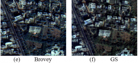
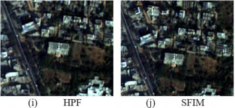
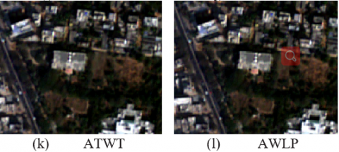
Figure 5. Images obtained by various pan sharpening methods
There is a pixel breakout or a stair-casing effect observed in all four MRA methods HPF, SFIM, ATWT and AWLP. Color variations observed in the methods Brovey, GS, PCA, PRACS, HPF and SFIM. Good contrast is observed for the methods IHS, Modified-IHS, Brovey, GS, and PRACS. From the Table 1, it is inferred that the most preferred feature extraction methods are IHS and modified IHS. The next preferred are Brovey, GS and PRACS methods. The least preferred methods are the two MRA methods HPF and SFIM because of this poor spatial quality.
Visual result of the same area (part of the resultant images) is provided in Figure 5.
5.2 Quantitative analysis
The spectral quality was more difficult to judge visually; therefore metrics were used to evaluate the results. The metrics used are CC-average, RMSE, PSNR, UIQ-average, ERGAS, SAM, SSIM, and Q4. After pan sharpening at 0.6 m resolution, the degraded MS dataset was produced at 1.6 m resolution, to compare it with the original MS image as per the widely accepted Wald’s method [22]. The results obtained are shown in Table 2(a) and (b).
It is observed that HPF and SFIM methods produced almost similar results. ATWT and AWLP methods also performed in a similar way. Low average CC, high RMSE, high ERGAS and poor SSIM values of wavelet-based methods show that structural information is lost hence least preferred. Major spectral quality indicators are matching for HPF and SFIM methods, (both are from the MRA family) hence they may be chosen for the applications that need spectral fidelity such as crop and vegetation analysis.
Table 2(a). Quantitative results of various pan sharpening methods
|
Parameter |
CC-avg |
RMSE |
PSNR |
UIQI-avg |
|
IHS |
0.9264 |
0.0768 |
35.9660 |
0.5349 |
|
Mod IHS |
0.9089 |
0.0619 |
36.5810 |
0.5596 |
|
BROVEY |
0.9241 |
0.0780 |
35.8282 |
0.5356 |
|
GS |
0.9182 |
0.0809 |
35.5105 |
0.5709 |
|
PCA |
0.9179 |
0.0811 |
35.4926 |
0.5678 |
|
PRACS |
0.9389 |
0.0740 |
35.2878 |
0.6834 |
|
HPF |
0.9977 |
0.0137 |
50.9494 |
0.9757 |
|
SFIM |
0.9976 |
0.0138 |
50.8840 |
0.9772 |
|
ATWT |
0.4231 |
0.2644 |
28.2359 |
0.0042 |
|
AWLP |
0.4231 |
0.2644 |
28.2339 |
0.0042 |
|
Requirement |
Higher better |
Lower better |
Higher better |
Higher better |
Table 2(b). Quantitative results of various pan sharpening methods
|
Parameter |
ERGAS |
SAM |
SSIM |
Q4 |
|
IHS |
5.6275 |
1.0311 |
0.9753 |
0.4314 |
|
Mod IHS |
4.9372 |
0.0935 |
0.9757 |
0.4841 |
|
BROVEY |
5.5508 |
~ 0 |
0.9752 |
0.4506 |
|
GS |
5.6858 |
1.9093 |
0.9755 |
0.5299 |
|
PCA |
5.6991 |
1.9263 |
0.9756 |
0.5302 |
|
PRACS |
5.0772 |
1.9459 |
0.9807 |
0.6439 |
|
HPF |
0.9706 |
0.3245 |
0.9999 |
0.974 |
|
SFIM |
0.9741 |
0.2974 |
0.9998 |
0.9754 |
|
ATWT |
13.3695 |
9.1029 |
0.6217 |
0.1549 |
|
AWLP |
13.3711 |
9.1005 |
0.6216 |
0.1549 |
|
Requirement |
Lower better |
Lower better |
Higher better |
Higher better |
However, as per the quantitative analysis, pixel breakings are more for the wavelet family methods. Hence, for automatic feature extraction, which involves edge detection, the modified-IHS provide higher fusion quality with less spectral distortion and also simultaneously conserving the spatial information. As PRACS method also is providing similar results, this method is suggested to be the next preferred / alternative to modified-IHS method.
Various pan sharpening methods are available for fusion of remote sensing images of high spatial resolution PAN image with low spatial and high spectral resolution MS image. The most suitable method for any particular data set depends on the characteristics of the sensor and its imaging technology. The suitable method is also based on the sensor and application for which it is being used.
In this paper, Component substitution methods such as IHS, Modified-IHS, Brovey, GS, PCA, PRACS and MRA methods like HPF, SFIM, AWLP and ATWT are applied on CARTOSAT-2E urban imagery. The quantitative and qualitative analysis shows that, the best methods for spectral quality fidelity are HPF and SFIM for this image. However, these methods suffer from stair-casing effect making them unusable for feature extraction. The suitable methods found to be modified-IHS followed by PRACS for urban feature extraction.
Future work may be carried out to find even better method by taking into account the imaging system’s modulation transfer function MTF.
[1] Strait, M., Rahmani, S., Markurjev, D. (2008). Evaluation of pan-sharpening methods. Tech. Rep., UCLA Department of Mathematics.
[2] Sarp, G. (2014). Spectral and spatial quality analysis of pan-sharpening algorithms: A case study in Istanbul. European Journal of Remote Sensing, 47(1): 19-28. https://doi.org/10.5721/EuJRS20144702
[3] Jawak, S.D., Luis, A.J. (2013). A comprehensive evaluation of PAN-sharpening algorithms coupled with resampling methods for image synthesis of very high resolution remotely sensed satellite data. Advances in Remote Sensing, 2(4): 332-344. https://doi.org/10.4236/ars.2013.24036
[4] Yang, J.H., Zhang, J.X., Huang, G.M. (2014). A parallel computing paradigm for pan-sharpening algorithms of remotely sensed images on a multi-core computer. Remote Sensing, 6(7): 6039-6063. https://doi.org/10.3390/rs6076039
[5] Amro, I., Mateos, J., Vega, M., Molina, R., Katsaggelos, A.K. (2011), Survey of classical methods and new trends in pan sharpening of multispectral images. EURASIP Journal on Advances in Signal Processing, 79. https://doi.org/10.1186/1687-6180-2011-79
[6] Kahraman, S., Ertürk, A. (2017). A comprehensive review of Pan sharpening algorithms for GÖKTÜRK-2 satellite images. ISPRS Annals of the Photogrammetry, Remote Sensing and Spatial Information Sciences, IV-4/W4: 263-270. https://doi.org/10.5194/isprs-annals-IV-4-W4-263-2017
[7] Presentation in NDC User Meet. (2017). Opportunities to Industries, ANTRIX Corporation Ltd. https://nrsc.gov.in /sites/all/pdf/Opportunities.pdf, accessed on Dec. 10, 2018.
[8] Otazu, X., González-Audícana, M., Fors, O., Núñez, J. (2005). Introduction of sensor spectral response into image fusion methods. Application to wavelet-based methods. IEEE Transactions on Geoscience and Remote Sensing, 43(10): 2376-2385. https://doi.org/10.1109/TGRS.2005.856106
[9] Choi, J., Yu, K., Kim, Y. (2011). A new adaptive component-substitution-based satellite image fusion by using partial replacement. IEEE Transactions on Geoscience and Remote Sensing, 49(1): 295-309. https://doi.org/10.1109/TGRS.2010.2051674
[10] Loncan, L. (2016). Fusion of hyperspectral and panchromatic images with very high spatial resolution. Signal and Image Processing. Université Grenoble Alpes, 2016. English. ⟨NNT: 2016GREAT065⟩.
[11] Li, H., Jing, L.H., Tang, Y.W. (2017). Assessment of Pansharpening methods applied to worldview-2 imagery fusion. Sensors, 17(1): 89. https://doi.org/10.3390/s17010089
[12] Loncan, L., Almeida, L.B., Bioucas-Dias, J.M., Briottet, X., Chanussot, J., Dobigeon, N., Fabre, S., Liao, W., Licciardi, G.A., Sim˜oes, M., Tourneret, J.Y., Veganzones, M.A., Vivone, G., Wei, Q., Yokoya, N. (2015). Hyperspectral pan sharpening: A review. IEEE Geoscience and Remote Sensing Magazine, 3(3): 27-46. https://doi.org/10.1109/MGRS.2015.2440094
[13] Vivone, G., Alparone, L., Chanussot, J., Mura, M.D., Garzelli, A., Licciardi, G.A., Restaino, R., Wald, L. (2015). A critical comparison among pan sharpening algorithms. IEEE Transactions on Geoscience and Remote Sensing, 53(5): 2565-2586. https://doi.org/10.1109/TGRS.2014.2361734
[14] Alparone, L., Baronti, S., Aiazzi, B., Garzelli, A. (2016). Spatial methods for multispectral pan sharpening: multi-resolution analysis demystified. IEEE Transactions on Geoscience and Remote Sensing, 54(5): 2563-2576. https://doi.org/10.1109/TGRS.2015.2503045
[15] Liu, J.G. (2000). Smoothing filter-based intensity modulation: A spectral preserve image fusion technique for improving spatial details. International Journal of Remote Sensing, 21(18): 3461-3472. https://doi.org/10.1080/014311600750037499
[16] Nunez, J., Otazu, X., Fors, O., Prades, A., Pala, V., Arbiol, R. (1999). Multiresolution-based image fusion with additive wavelet decomposition. in IEEE Transactions on Geoscience and Remote Sensing, 37(3): 1204-1211. https://doi.org/10.1109/36.763274
[17] Yuhas, R.H., Goetz, A.F.H., Boardman, J.W. (2013). Discrimination among semi-arid landscape end members using the spectral angle mapper (SAM) algorithm. Publication: JPL, Summaries of the Third Annual JPL Airborne Geoscience Workshop. Volume 1: AVIRIS Workshop.
[18] Jagalingam, P., Hegdeb, A.V. (2015). A review of quality metrics for fused image. Aquatic Procedia, 4: 133-142. https://doi.org/10.1016/j.aqpro.2015.02.019
[19] Mercovich, R.A. (2015). Evaluation techniques and metrics for assessment of pan+MSI fusion (pan sharpening). Proc. SPIE 9472, Algorithms and Technologies for Multispectral, Hyperspectral, and Ultra spectral Imagery XXI, 94721I (21 May 2015). https://doi.org/10.1117/12.2177093
[20] Wang, Z., Bovik, A.C. (2002). A universal image quality index. IEEE Signal Processing Letters, 9(3): 81-84. https://doi.org/10.1109/97.995823
[21] Pendyala, V.G.K., Kalluri, H.K., Rao, C.V. (2019). Dense DSM and DTM point cloud generation using CARTOSAT-2E satellite images for high-resolution applications. Journal of the Indian Society of Remote Sensing, 47(12): 2085-2096. https://doi.org/10.1007/s12524-019-01051-0
[22] Wald, L., Ranchin, T., Mangolini, M. (1997). Fusion of satellite images of different spatial resolutions: Assessing the quality of resulting images. Photogrammetric Engineering & Remote Sensing, 63(6): 691-699.