Tulasi Krishna Sajja* | Hemantha Kumar Kalluri
OPEN ACCESS
In this paper, presented a Gender classification through Support Vector Machine (SVM) and Scaled Conjugate Gradient Back Propagation Neural Network (SCGBPNN) from face images using Local Binary Patterns. To achieve better classification performance, need to be applied pre-processing technique first and then extracted the features on facial images from Local Binary Pattern Histogram (LBPH) method. These extracted features were stored into a vector called feature vector. Later, the feature vector is inputted to Polynomial SVM and SCG Back Propagation Neural Network classification methods along with labelled target vector. The performance of the both classifiers is measured by the labelled AT&T face database and Nottingham Scan Database.
Local Binary Pattern (LBP), pattern recognition, scaled conjugate gradient back propagation Neural Network (SCG), Support Vector Machine (SVM)
Now-a-days face Biometrics is most commonly used to recognize human faces in various applications. Most of the applications use face trait for the security purposes, such as criminal activities, forensic etc. The aim of the face recognition system is to recognize a given face from a database where images are stored. Feature extraction and classification are the two main steps in face recognition. LBPH [1-2] (Local Binary Pattern histogram) is used for extracting the features from facial images. SVM [3-5] (Support Vector Machine) and NN (Neural Networks) both are supervised learning. SVM is the most common method for classification. SCG is fully automated which include no crucial user-dependent parameters and avoids time consuming [6].
Karanwal S et al. [1] have been proposed Local Binary Pattern Histogram (LBPH) and Local Binary Pattern Image (LBPI). Further, Yekkehkhany B. et al. [3] explained about the different SVM kernel algorithms such as polynomial, sigmoid, Radial Basis Function. Nisha et al. [7] have used circular Local binary patterns for feature extraction and Support Vector Machine (SVM) is used for image classification. With these methods researchers got 94.33 %. Saini et al. [8] used LBP and SVM they achieved 88.75 %. Nandini et al. [9] achieved 98.88 % with the Back Propagation Neural Network (BPN) andaRadialaBasisqFunction (RBF). Datta et al. [10] have proposed texture based Local Binary Pattern for feature extraction and the learning algorithms applied such as Naïve Bayes, K-Nearest Neighbor, Linear SVM and Artificial Neural Network (ANN). The researchers got 84 % and 63 % respectively. The literature survey shows, there is a need to improve the gender classification accuracy using face images.
The remaining part of the manuscript is organized asdfollows:a Section-2 explains about the Local Binary Patterns Histogram (LBPH) for feature extraction. Section-3 describes the supervised learning methods such as Polynomial SVM and Scaled Conjugate Gradient back propagation Neural Network. Section-4 explains the proposed procedure for classification. Section-5 shows the experimental results and conclusion are highlighted inqSection-6.
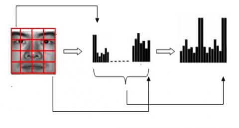
Local Binary Pattern (LBP) is an efficient feature extraction method, which gives the same size of the original image with decimal values instead of gray pixel values. The combination of LBP with histograms [1] represents the face images as a data vector. The original face image is divided into local regions and LBP texture descriptors are extracted from each region independently, which is shown in Figure 1.
The following procedure is needed to get the feature descriptor from the original image region.
(1). Input face image is converted into gray image.
(2). Take the part of region as a window of 3x3 pixel.
(3). With each 3x3 pixels, centre pixel value is compared with its eight-neighbours then if the neighbour values are greater than the centre pixel value place 1, otherwise place 0.
Figure 1. Procedure for extracting LBP code from the face region part
(1). From each 3x3 pixel, acquired eight-bit binary number. The generated binary number is called LBP code.
(2). Convert LBP code into decimal value.
(3). Then, the decimal value and set it to the central value of the matrix, which is actually a pixel from the original image.
(4). Repeat the same procedure for all parts of the region in face image and find LBP code for that region.
(5). Then generate the histogram for that region.
The descriptors extracted from each region are concatenated using histogram to form a global histogram of the face. Repeat the above procedure for all regions to find the histograms of each region, the final histogram is shown in Figure 2.
The generated histograms contain 256 bins, the occurrences of each pixel intensity. As per the experiment requirement we captured the occurrences of the pixels intensity with 10 bins instead of 256 bins. Then the feature vector is generated with final histogram.
Figure 2. Final Histogram generated for face image
3.1 Support vector machine
Support Vector Machine (SVM) [3-5] is one of the most commonly used classifiers. It is easy to represent the linear hyper-plane between two classes. But in some cases we could not separate the two classes, for this, SVM choose a kernel trick technique, which transforms the data from lower dimensional input space to higher dimensional space. Now separate the two classes from Non-separable problem. Many kernels are used by the SVM classifier; those are Sigmoid, Polynomial and Gaussian Radial Basis Functions (RBF) [11, 12]. In experiment we used polynomial function for classification.
Kernel function is defined as:
$k(\bar{x})=\begin{array}{rl} 1 & \text{if } ||\bar{x}||\leq 0,\\ 0 & \text{otherwise}. \end{array}$ (1)
SVM with Polynomial Kernel function:
The Polynomial SVM [3,5] function is also called as Non-Linear function. By applying kernel function the hyper plane drawn with a maximum margin in a higher dimensional plane.
$k(\bar{x_i},\bar{x_j})=(\bar{x_i},\bar{x_j})^d$ (2)
where $k(\bar{x_i},\bar{x_j})$ is a Kernel function, $x_i,x_j$ are feature vectors and d is the degree of polynomial equation.
3.2 SCG BP neural network
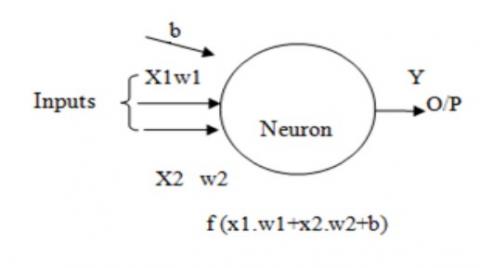
An Artificial Neural Network (ANN) is an outstanding network which is inspired by the biological Neural Networks in the human brain. The important unit for computing in a Neural Network is Neuron or node, which receives input from external sources for computing output. Every input is associated with weight (w); the node applies a function (f) to the weighted sum of its inputs as:
Figure 3. Single neuron
The output is calculated from the neuron is shown in the Figure 3. The function is called the Activation Function because it is Non-linear. The reason to use in real world is non-linear. Out of several Activation Functions we used sigmoid Activation Function; its value is in between 0 and 1.
Sigmoid function:
$\sigma (x)=1/(1+e^{-x})$ (3)
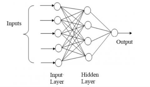
The General Architecture of the Neural Network is shown in Figure 4. It has one input Layer, one or more hidden Layers and one Output Layer. Neural Networks are divided into many types and subtypes. One is Feed-Forward Neural Network (FFNN) and the other is Recurrent Neural Network (RNN) [13]. There are two subtypes in FFNN is Single Layer Perceptron (SLP), which has no hidden layers and it learned linear functions. The second one is Multi-Layer Perceptron (MLP) [14] which has one or more hidden layers and learns non-linear functions. The process by learning through MLP is called back propagation algorithm. Back Prop is one of the ways to learn from data and error propagation. The experiment results were taken from Feed Forward Neural Network of MLP. This FFNN network trained with Scaled Conjugate Gradient back propagation Neural Network (SCG) [15].
Figure 4. General architecture of artificial neural network
As per the experimental requirement, AT & T database is re-organized as male and female labelled database. To remove noise from the images, adjusting the lightening conditions applied pre-processing techniques. Histogram equalization pre-processing technique gave better enhancement on face images, because AT & T database images are undergone pose, illumination variations under different lightening conditions. From the pre-processed images we extracted the features by using Local Binary Pattern Histogram (LBPH) algorithm which is explained in Section-2. The histograms of each region of LBP algorithm concatenated and formed the feature vector of the database images. This feature vector is inputted to the both learning algorithms (SVM and SCGBPNN).
SVM: The feature vector is inputted to SVM system and set the target labels for input data because SVM is supervised learning. Before splitting, training and testing data we need to standardize the data, because SVM tries to maximize the distance between the support vectors and the separating plane. If one dimension in this space has large values, it will influence on the other dimensions while distance Calculating phase. If we standardize all dimensions (e.g. to [0, 1]), they all will have the same nature on the distance calculation metric. Then split 60 % train and 40 % test data, gives the strong fit, otherwise increasing training samples causes over fitting. After splitting, train the system with splitted data for good learning. Then test the system with test data. Repete the process with different train and test samples. The experimental results are placed in Table 1.
SCGBPNN: A neural network is used to classify the input data with a set of target data. A two layer feed-forward network, consists hidden nodes and output neurons with sigmoid Activation function could classifies the input data. The network trained with scaled conjugate gradient back propagation neural network after split the 60 % training data and 40 % testing data.
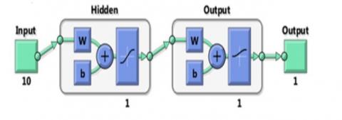
In experiment, the system train with ten input neurons, because the feature vector generated with ten discriminated features for each image. We have taken only one hidden layer for computation. The proposed network architecture is shown in Figure 5(a). Train the proposed network, if got any errors, retrained the proposed network with multiple times until the Cross-Entropy and Error percentage minimized. The performance curve of NN is shown in Figure 5(b).
(a) Neural network
(b) Performance curve
Figure 5. Network with performance graph
5.1 AT & T database
AT & T Database [16] is popularly known as ORL Database. The ORL Database contains740adistinct subjects. Each subject hasa10 different human face images with lighting variations, time taken, facial expressions and face details. All the images are in pgm format extension and the size of each image in dataset is contains 360 images and female database contains 40 images. The sample male and female faces from re-arranged database are shown in Figure 6.
Table 1. Comparisons between the SVM and Neural Network Performance on ORL Database
|
No.of Images |
LBP+SVM |
LBP+ back propagation Neural Network (SCG) |
|||
|
Training |
Testing |
Accuracy (%) |
Sensitivity (%) |
Accuracy (%) |
Sensitivity (%) |
|
30 % 120 images |
70 % 280 images |
89.29 |
100 |
100 |
100 |
|
60 % 240 images |
40 % 160 images |
93.75 |
100 |
100 |
100 |
|
70 % 280 images |
30 % 120 images |
100 |
100 |
100 |
100 |
|
S.No |
Existing Methods and Results |
Accuracy of Proposed method |
||||||
|
REFERENCE |
Method Used |
Data base used |
Train Images (%) |
Test Images (%) |
Accuracy of existing method |
LBP+SVM |
LBP+NN |
|
|
1 |
Nisha et al. [7] |
LBP+SVM |
ORL |
75 |
25 |
94.33 % |
100 % |
100 % |
|
2 |
Saini et al. [8] |
LBP+SVM |
ORL |
60 |
40 |
88.75 % |
93.75 % |
100 % |
|
3 |
Nandini et al. [9] |
BPN+RBF |
ORL |
70 |
30 |
98.88 % |
100 % |
100 % |
|
4 |
Datta et al. [10] |
LBP+ANN |
Nottingham Scan Database |
80 |
20 |
63 % |
55 % |
71 % |
Figure 6. Sample male and female faces of ORL database
5.2 Nottingham scan database
Nottingham Scan database [17] contains 100 human faces. Among hundred faces, 50 face images are Male and 50 face images are Female. All the images are in .gif format and the size of each image in this dataset is 438x538 pixels, with 256agrayalevels. As per the requirement of the experiment, cropped each image of the database. The sample Nottingham male and female faces are shown in Figure 7.
Figure 7. Sample cropped male and female faces of Nottingham database
5.3 Results and discussion
5.3.1 Performance metrics
The researchers can evaluate the efficiency and performance of learning algorithms by considering the factors [18]. The accuracy of an algorithm is determined by using a confusion matrix. Sensitivity and Specificity are measures of the binary classification algorithms.
5.3.2 Experimental outputs
The performance measures of the SVM and Neural Network are tabulated in Table 1. Out of 400 images 30 % images are taken as training and 70 % images for testing, indicates 1204images are used for training and 280 images are for testing, then we got 89.29 % accuracy with SVM classifier, and on same testing and training images Artificial Neural Network (ANN) achieved 100 % accuracy. Thereafter, we inputted with different training and testing images and it gives better results. The system learned with 60 % training and 40 % testing is recommended, above than this training percentage of images, over fitting problem occurs.
Nisha et al. [7] have used circular Local binary patterns for feature extraction and SVM is used for classifying, using these methods they split 75 % training data and 25 % testing data, achieved 94.33 %, but with our SVM and NN methods we got 100 %, 100 % respectively. The results are given in Table 2. Saini et al. [8] used LBP and SVM and achieved 88.75 % accuracy with training and testing as 60:40 ratio, we got 93.75 % and 100 % respectively. Nandini et al. [9] achieved 98.88 % with the Back Propagation Neural Network (BPN) and Radial Basis Function (RBF), the researchers divide 70 % training and 30 % testing images, we got100% in both cases. The results are placed in Table 1.
Datta et al. [10] have used texture based Local Binary Pattern for feature extraction and the learning algorithms applied like naïve Bayes, Linear SVM and Artificial Neural Network (ANN) etc. The researchers got 63 % for ANN classification algorithm, but with our proposed method, the combination of LBP and SVM got 55 % and combination of LBP and NN got 71 % by using the Nottingham Scan database shown in Table 2.
In this paper, we extracted the features using LBPH method after pre-processing stage. After that Classification is performed by using polynomial SVM and Scaled Conjugate Gradient Neural Network for gender classification. From the experimental results, it has been found, that the combination of LBP and Neural Networks have better performance than the combination of LBP and polynomial SVM. By using the combination of LBP and Neural Network we got 100 % accuracy with ORL database, and also by using the combination of LBP and Neural Network we got 71 % accuracy with Nottingham database. The experimental results show that the proposed method provides better results compared with the earlier researchers [7-10].
[1] Karanwal, S., Purwar, R.K. (2017). Performance analysis oflocal binary pattern features with PCA for face recognition. Indian Journal of Science and Technology, 10(23): 1-10. https://doi.org/10.17485/ijst/2017/v10i23/115561
[2] Heni, B., Yassine, R. (2018). Deep feed forward neural network learning using local binary patterns histograms for outdoor object categorization. Advances in Modelling and Analysis B, 61(3): 158-162. https://doi.org/10.18280/ama_b.610309
[3] Yekkehkhany, B., Safari, A., Homayouni, S., Hasanlou, M. (2014). A comparison study of different kernel functions for SVM-based classification of multi-temporal polarimetry SAR data. The International Archives of Photogrammetry, Remote Sensing and Spatial Information Sciences, 40(2): 281-285. https://doi.org/10.5194/isprsarchives-XL-2-W3-281-2014
[4] Chen, R., Cao, Y., Sun, H., Yang, W. (2008). A modified method for face recognition using SVM. International Journal of Intelligent Engineering and Systems, 22-29. https://doi.org/10.22266/ijies2008.0331.04
[5] Wang, H., Xu, D. (2017). Local capability analysis and comparative study of kernel functions in support vector machine. AMSE JOURNALS-AMSE IIETA Publication-2017-Series: Advances B, 60(2): 338-356. https://doi.org/10.18280/ama_b.600206
[6] Møller, M.F. (1993). A scaled conjugate gradient algorithm for fast supervised learning. Neural Networks, Elsevier, 6(4): 525-533. https://doi.org/10.1016/S0893-6080(05)80056-5
[7] Nisha, M.D. (2017). Improving the recognition of faces using LBP and SVM optimized by PSO technique. International Journal of Engineering Development and Research, 5(4): 297-303.
[8] Saini, P.K., Banerjee, S., Durrani, V. (2017). Comparative analysis of LBP variants in FACE recognition application using SVM. International Journal of Innovations & Advancement in Computer Science, 316-325.
[9] Nandini, M., Bhargavi, P., Sekhar, G.R. (2013). Face recognition using neural networks. International Journal of Scientific and Research Publications, 3(3): 1-5.
[10] Datta, S., Das, A.K. (2015). Gender identification from facial images using local texture based features, 1-5. https://samyak-268.github.io/pdfs/gender-report.pdf
[11] Chittora, A., Mishra, O. (2012). Face recognition using RBF kernel based support vector machine. International Journal of Future Computer and Communication, 1(3): 280-283. https://doi.org/10.7763/IJFCC.2012.V1.75
[12] Gaddam, V.G., Babu, G.R.M. (2018). Tolerable kernel service in support vector machines using distribution classifiers. Advances in Modelling and Analysis B, 61(1): 23-27. https://doi.org/10.18280/ama_b.610105
[13] Kasar, M.M., Bhattacharyya, D., Kim, T.H. (2016). Face recognition using neural network: A review. International Journal of Security and Its Applications, 10(3): 81-100. https://doi.org/10.14257/ijsia.2016.10.3.08
[14] Al-Allaf, O.N. (2014). Review of face detection systems based artificial neural networks algorithms. The International Journal of Multimedia & Its Applications (IJMA), 6(1): 1-16. https://doi.org/10.5121/ijma.2013.6101
[15] Utomo, D. (2017). Stock price prediction using back propagation neural network based on gradient descent with momentum and adaptive learning rate. Journal of Internet Banking and Commerce, 22(3): 1-16.
[16] [Online] [AT & T database] http://www.cl.cam.ac.uk/research/dtg//attarchive/facedatabase.html/
[17] [Online][Nottingham Scan Database] hhttp://pics.stir.ac.uk/2D_fӓce_sets.html/
[18] Ramteke, S.P., Gurjar, A.A., Deshmukh, D.S. (2018). A streamlined OCR system for handwritten marathi text document classification and recognition using SVM-ACS algorithm. International Journal of Intelligent Engineering and Systems, 11(3): 186-195. https://doi.org/10.22266/ijies2018.0630.20