Arnold Mauduit* | Hervé Gransac
© 2020 IIETA. This article is published by IIETA and is licensed under the CC BY 4.0 license (http://creativecommons.org/licenses/by/4.0/).
OPEN ACCESS
The precipitation kinetics and mechanisms of 6000 series aluminium alloys (6082 and 6061 alloys) are studied through the changes in the electrical conductivity. This is supplemented by hardness measurements. The Johnson – Mehl – Avrami – Kolmogorov (JMAK) and Austin – Rickett (AR) models are applied to the results of the electrical conductivity measurements carried out on the two aluminum alloys allowing their parameters to be identified. These two models offer a good representation of the precipitation kinetics of the two aluminum alloys. They were also used to calculate the activation energies for the transformations by applying the Arrhenius equation. The activation energies obtained are consistent with the data in the literature. Finally, two partial time – temperature – precipitation (TTP) diagrams are created for the 6082 and 6061 alloys. A comparison of the information obtained from these diagrams and the Transmission Electron Microscopy (TEM) examinations is proposed for these two aluminium alloys and thus makes it possible to find a good match.
electrical conductivity, precipitation kinetics, 6000 series aluminium alloys
The experimental methods for studying the structural precipitation of aluminium alloys include macroscopic physical methods which analyse macroscopic changes in the physical properties (electric, thermal, dimensional, etc.) of the aluminium alloy as a function of its precipitation state [1]. The electrical conductivity and conversely the electrical resistivity are governed by the progress of the solid solution breakdown of the studied aluminium alloy. Consequently, the electrical conductivity measurement at room temperature is already being used in the aerospace industry, among others, as a quick non-destructive method for testing quenched and tempered semi-products made from aluminium alloys.
The study of the precipitation kinetics is associated with the nucleation and growth processes which are predominant in supersaturated aluminium alloys. The kinetics of isothermal phase transformations through nucleation and growth have often been described by the Johnson – Mehl – Avrami – Kolmogorov (JMAK) model [2-5] which postulates that nucleation occurs randomly and that growth is homogenous, or the Austin – Rickett (AR) [6] model which is sometimes more suited to controlled diffusion precipitation reactions.
In this study, a detailed presentation is proposed of the electrical conductivity measurement method as well as the models used to describe the precipitation kinetics. Both models are compared and analysed to calculate the transformation activation energies. All the data acquired during the study is ultimately used to construct partial time – temperature – precipitation (TTP) diagrams.
The overall approach is implemented on two structural hardening aluminium alloys of the 6000 series: 6082 and 6061. This family of alloys is typified by the addition of two main elements, namely magnesium (Mg) and silicon (Si). In general, 6000 series alloys exhibit good hot forming capacities (e.g. extrusion), good corrosion resistance as well as a fairly good level of mechanical properties which may be improved by adding Cu (e.g. 6061 alloy).
2.1 Aluminium alloys: 6082 and 6061
The EN AW-6082 [AlSi1MgMn] alloy is used in the T6 temper. In this state, it provides an excellent balance between the relatively high mechanical characteristics, greater than those of 6061 T6, good corrosion resistance and acceptable weldability. This alloy is used to make laminated, extruded (bars, tubes, profiled sections) and forged products.
The 6082 alloy with a large excess of Si compared with the pseudo-binary Al-Mg2Si mixture of the Al-Si-Mg phase diagram has the following sequence of precipitation [1, 7]:
Initial solid solution → Clusters of Mg and Si → Guinier-Preston (GP) zones → β’’ → β’ → β (Mg2Si).
The EN AW-6061 [AlMg1SiCu] alloy also exhibits excellent capacity for deformation in the annealed (O) and freshly quenched state and the thus formed products must then be heat treated to be used in the T6 condition where the alloy offers a good compromise of properties between average mechanical properties, good corrosion resistance and appropriate weldability. This alloy is used to make laminated, extruded (bars, profiled sections, tubes), drawn or forged products.
The 6061 alloy tends to have excess magnesium and furthermore a low percentage of Cu is added, thereby slightly modifying the sequence of precipitation as follows [1, 7, 8]:
Initial solid solution → Cluster of Mg and Si → Guinier-Preston (GP) zones → β’’ → β’ + B’ → β (Mg2Si).
According to the ageing peak of the Al-Mg-Si-Cu alloys, some needle-like β’’ precipitates are replaced by rod-like β’ precipitates and others are replaced by lath-like precipitates. These lath-like precipitates were originally observed in the 6061 alloy and were called B’ precipitates. The B’ (or Q’) phase is now considered as the forerunner of the Q phase which is commonly encountered in Al-Cu-Mg-Si [7, 8] type alloys.
The aluminium alloy specimens used in the study were made from 10 mm thick laminated sheets in the case of the 6082 alloy and 1.2 mm thick laminated sheets for the 6061 alloy.
The chemical composition and the mechanical characteristics of these two alloys comply with standards EN 573-3 and EN 485-2.
2.2 Measurement method
2.2.1 Material equipment
To measure the electrical conductivity of non-magnetic metals (as in the case of aluminium alloys), we use the Eddy current method. The instrument used is a Fisherscope MMS pc equipped with an ES40 probe.
The Brinell hardness measurements (HBW 5/250) are carried out at room temperature (20±2℃) on a Duramin 500 Emco-test hardness tester (as per standard NF EN ISO 6506‑1).
The samples intended for the transmission electron microscopy (TEM) examinations are prepared by mechanical polishing (for thinning) then via ionic abrasion using a Precision Ion Polishing System (PIPS). The TEM is a Tecnai Osiris (200 kV).
We use a forced convection air oven (N15/65HA model – Nabertherm) to carry out the heat treatments. This oven is designed for the treatments of aluminium alloys (≤ 650℃) and features excellent temperature uniformity (ΔT ≤ 6℃). The quenching fluid is cold water (≈ 20℃). The transfer time of the load (specimens) in the quenching medium is less than 5 seconds in all cases.
2.2.2 Experimental methods
The study is largely based on the quality and reliability of the electrical conductivity measurements, so we indicate the necessary recommendations to adopt for them.
To limit the edge effects [9], the minimum diameter recommended by the manufacturer of the probe to carry out the measurements is 11 mm. The minimum diameter used during the test is approximately 18 to 20 mm.
The temperature of the sample has a significant impact on the electrical conductivity measurements. The physical correlation between the electrical conductivity and the temperature of the sample is described by the following equation [9, 10]:
$\sigma=\frac{\sigma_{20}}{1+\alpha(T-20)}$ (1)
where,
$\sigma$ : electrical conductivity in MS/m
$\sigma_{20}$ : electrical conductivity at 20℃
T: temperature of the sample in ℃
$\alpha$ : temperature coefficient of the electrical conductivity for the sample
The reference temperature of the electrical conductivity is 20℃. For example: it can be seen that if the temperature increases by only 2℃, the measured electrical conductivity of the pure copper decreases by 0.46 MS/m (which is a significant proportion) [9].
All our tests are carried out at 22±2℃. To limit measurement errors from temperature changes, we use the ES40 probe in its compensation function. This means that the probe and the measurement equipment automatically compensate or correct the electrical conductivity [9]. As a matter of fact, the ES40 probe is equipped with a thermocouple to take the temperature of the sample and the Fischer scope MMS pc automatically recalculates the $\alpha$ coefficient as a function of the temperature measured by the probe and instantly corrects the electrical conductivity. The values subsequently presented are therefore $\sigma_{20}$.
We use a frequency of 60 kHz to penetrate as deep as possible within the alloy. However, the thickness of the specimens must not be excessively low as this would create errors. Furthermore, the probe has the best repeatability accuracy with this frequency (less than 0.06 MS/m) [9].
The amplitude of the Eddy currents decreases exponentially with the penetration depth. The depth at which the amplitude is approximately 37% of that of the surface is called the standard penetration depth $\delta$ [10].
Let us calculate the standard penetration depth $\delta$ for the selected aluminium alloys [10]:
$\delta=\frac{503.3}{\sqrt{f \sigma}}$ (2)
where,
$\delta$: standard penetration depth in mm
f: frequency selected for the measurement in Hz (in this case 60 kHz)
$\sigma$ : electrical conductivity of the sample in MS/m
For the studied aluminium alloys, it will be seen that the electrical conductivity varies between 24 MS/m and 30 MS/m hence $\delta$= 0.375 mm to 0.42 mm. If the thickness of the test sample is more than 2.6 $\delta$, then the effect of the thickness is negligible on the Eddy currents and therefore on the electrical conductivity measurement. Thus, the minimum thickness of the samples must be 0.975 mm to 1.1 mm depending on the electrical conductivity of the alloy; this is consistent with the thicknesses of the samples used (paragraph 2.1.).
The calibration is carried out with two reference standards [9]:
- an electrical conductivity standard at 60kHz and 20°C of 14.46 MS/m
- an electrical conductivity standard at 60kHz and 20°C of 34.69 MS/m
These reference standards encompass all the electrical conductivity measurements carried out on the aluminium alloys.
For each aluminium alloy, the electrical conductivity is measured in the configurations shown in Table 1.
A mean is calculated based on 5 electrical conductivity measurement points.
To complete the electrical conductivity measurements, a few hardness tests are also carried out.
Table 1. Configurations of heat treatments followed by electrical conductivity
|
Heat treatment |
Measured at |
|
Isothermal transformation at room temperature (20±2°C) or natural ageing up to T4 state (after solution heat treatment and water quenching) |
5 min – 10 min – 15 min – 30 min – 1 h – 2 h – 4 h – 8 h – 24 h – 48 h – 72 h – 96 h – 168 h |
|
Isothermal transformation at a temperature of 135°C – 165°C – 190°C – 210°C (after solution heat treatment, water quenching and natural ageing of 48 hours) |
|
|
Annealing (404°C for 2 to 3 hours) |
Approximately 30 min |
The JMAK model is based on the concept of an “extended volume” which is the volume hat a new nucleus would occupy if there was no encroachment or overlapping of an already transformed adjacent nucleus [2-5, 11].
The JMAK equation is:
$x(t)=1-\exp \left(-[k(T) t]^{n}\right)$ (3)
where,
x(t) is the transformed volume fraction.
n is the Avrami exponent which reflects the transformation mechanism [12-14].
t is the isothermal hold time.
k(T) is a rate constant which primarily depends on the temperature and which may be expressed by an Arrhenius equation:
$k(T)=k_{0} \exp \left(-\frac{E_{a}}{R T}\right)$ (4)
where, $E_{a}$ is the activation energy for the nucleation and isothermal growth, k0 is a constant and R is the universal gas constant.
Austin and Rickett propose another model [6]:
$x(t)=1-\left(\frac{1}{[k(T) t]^{n}+1}\right)$ (5)
As mentioned in the introduction, this model is more suited to controlled diffusion precipitation reactions.
Electrical conductivity is governed by the progress of breakdown of the solid solution of the aluminium alloys and therefore by the transformation kinetics (precipitation and dissolution of the precipitates).
Thus, the transformed volume fraction of an isothermal reaction can be described as follows [15, 16]:
$x(t)=\frac{\sigma(t)-\sigma_{0}}{\sigma_{f}-\sigma_{0}}$ (6)
where,
x(t): transformed volume fraction at time t (isothermal transformation)
$\sigma(t)$: electrical conductivity at time t
$\sigma_{0}$: initial electrical conductivity
$\sigma_{f}$ : final electrical conductivity
3.1 Results of the electrical conductivity and hardness measurements
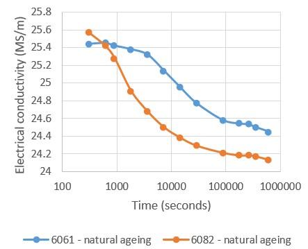
Figure 1 shows the monitoring by electrical conductivity of the natural ageing of the 6082 and 6061 alloys, i.e. the isothermal transformation at room temperature (approximately 22℃) to the stable T4 state.
Figure 1. Changes in the electrical conductivity during the natural ageing of the 6082 and 6061 alloys
A decrease in the electrical conductivity can be noted for both alloys. This decrease stabilises after several days (approximately 7 to 8 days i.e. 604,800 seconds to 691,200 seconds): the stable T4 state is therefore achieved. A natural ageing period of minimum 8 days is recommended for these alloys [17] which is consistent with Figure 1. There is a more rapid decrease in the electrical conductivity for the 6082 alloy: the natural ageing starts immediately whereas with the 6061 alloy, an incubation period of approximately 30 minutes is observed.
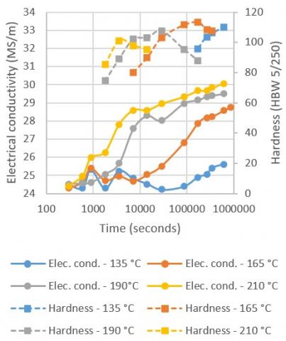
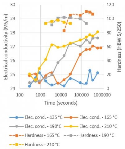
Figures 2 and 3 show the changes in the electrical conductivity and hardness at various temperatures (Table 1) during the artificial ageing operations (isothermal) from the T4 state (after natural ageing) for both the 6082 and 6061 alloys.
Figures 2 and 3 yield the following comments:
Figure 2. Changes in electrical conductivity and hardness during the various isothermal transformations from the T4 state – 6082 alloy
Figure 3. Changes in the electrical conductivity and hardness during the various isothermal transformations from the T4 state – 6061 alloy
3.2 Application of the JMAK and AR models
The transformed volume fraction at time t: x(t) may be obtained from the electrical conductivity measurements presented above using the Eq. (6). Following this, the parameters of the JMAK and AR models can be determined based on Eqns. (3) and (5) as follows:
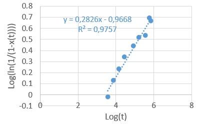
$\log \left(\ln \left(\frac{1}{1-x(t)}\right)\right)=\operatorname{nlog} t+\operatorname{nlog}(k(T))$ (7)
Therefore, we simply plot $\log \left(\ln \left(\frac{1}{1-x(t)}\right)\right)$ as a function of $\log t$. If the model applies, then we must obtain a line (possibly line segments). In this case, n the Avrami exponent is the slope of the line and $\operatorname{nlog}(k(T))$ is the intercept point. We obtain n and k(T).
Using the Arrhenius equation, we can obtain the activation energy $E_{a}$ based on Eq. (4):
$\ln (k(T))=\ln k_{0}-\left(\frac{E_{a}}{R T}\right)$ (8)
$E_{a}$ is therefore the slope of the line.
$\ln \left(\frac{1}{1-x(t)}-1\right)=n \ln t+n\ln (k(T))$ (9)
Therefore, we simply plot $\ln \left(\frac{1}{1-x(t)}-1\right)$ as a function of lnt. If the model applies, then we must obtain a line (possibly line segments). In this case, n is the slope of the line and nln(K(T)) is the intercept point. As for the JMAK model, we obtain n and k(T).
If we use the Arrhenius equation in the same way, we obtain the activation energy Ea.
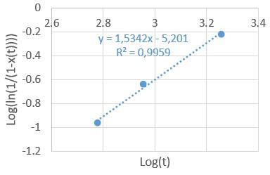
An example of the approach for the 6082 alloy is presented in Figures 4 and 5 during the isothermal transformation at room temperature, i.e. during natural ageing.
Figure 4. Application of the JMAK and AR models during natural ageing – 6082 alloy
In Figure 4, we obtain for the two models (JMAK and AR) two line segments: the models can therefore be applied as previously specified. It also shows that the natural ageing takes place in two transformations.
Based on these two line segments, we can therefore obtain for each of the two transformations: n (slope of the line segment) and k(T) (nlog(K(T)) is the intercept point) as represented on Figure 5 a – b for the JMAK model.
Table 2. Parameters identified for the JMAK and AR models – 6082 and 6061 alloys
|
Aluminium alloy 6082 |
||||||||
|
JMAK |
Artificial ageing |
Natural ageing |
||||||
|
Temperature (°C) |
165 (1) |
165 (2) |
190 (1) |
190 (2) |
210 (1) |
210 (2) |
RT (1) |
RT (2) |
|
n |
0,816 |
0,217 |
1,12 |
0,213 |
1,185 |
0,182 |
1,53 |
0,283 |
|
K(T) x10-5 |
0,503 |
2,25 |
6,45 |
2,01 |
22,4 |
10,4 |
40,7 |
37,9 |
|
AR |
Artificial ageing |
Natural ageing |
||||||
|
Temperature (°C) |
165 (1) |
165 (2) |
190 (1) |
190 (2) |
210 (1) |
210 (2) |
RT (1) |
RT (2) |
|
n |
0,887 |
0,383 |
1,67 |
0,363 |
1,115 |
0,414 |
1,78 |
0,703 |
|
K(T) x10-6 |
6,77 |
8,90 |
126 |
92,7 |
277 |
210 |
506 |
595 |
|
Aluminium alloy 6061 |
||||||||
|
JMAK |
Artificial ageing |
Natural ageing |
||||||
|
Temperature (°C) |
165 (1) |
165 (2) |
190 (1) |
190 (2) |
210 (1) |
210 (2) |
RT (1) |
RT (2) |
|
n |
1,24 |
0,058 |
1,11 |
0,158 |
0,98 |
0,158 |
1,03 |
0,223 |
|
K(T) x10-5 |
0,698 |
0,0004 |
4,28 |
0,243 |
20,4 |
0,779 |
4,55 |
27,0 |
|
AR |
Artificial ageing |
Natural ageing |
||||||
|
Temperature (°C) |
165 (1) |
165 (2) |
190 (1) |
190 (2) |
210 (1) |
210 (2) |
RT (1) |
RT (2) |
|
n |
1,15 |
0,080 |
1,19 |
0,239 |
1,195 |
0,245 |
1,21 |
0,615 |
|
K(T) x10-5 |
0,658 |
0,224 |
5,31 |
2,36 |
29,6 |
7,40 |
6,43 |
23,9 |
(2) 2nd transformation kinetics, i.e. second line segment
RT means Room Temperature
(a) First transformation kinetics
(b) Second transformation kinetics
Figure 5. Determination of n and k(T) for the JMAK model during natural ageing – 6082 alloy
Table 3. Representation of the Avrami exponent on the transformation kinetics
|
Diffusion-controlled transformations |
|
|
Morphology |
n |
|
Spheres Needles and/or spaced plates Thickening of the needles Thickening of the plates |
1.5 1 1 0.5 |
The same approach is applied for the isothermal transformations at 165℃, 190℃ and 210℃ with the JMAK and AR models for the 6082 and 6061 alloys. The results are provided in Table 2.
The Avrami exponent n can be associated with a precipitation morphology during a transformation as shown in Table 3 [12-14].
Tables 2 and 3 can be used as a basis to discuss the transformation kinetics observed on the 6082 and 6061 alloys.
3.2.1 6082 alloy
With the JMAK model, during natural ageing at room temperature, two values of n can be seen which suggest two transformation reactions. Firstly, there is n = 1.5 (approximately) which means that the transformation is controlled by diffusion and that the precipitates have a sphere-type morphology [12, 14, 16]. Over time, n decreases to a value of approximately 0.3. This suggests that diffusion-controlled transformation has continued but that the precipitates are thickening of plate-like precipitates [12, 14]. Drawing on paragraph 2.1 regarding the precipitation sequence of the 6082 alloy, the initial solid solution firstly breaks down into clusters of Mg and Si atoms which can be likened to spheres. This is followed by the fine needle-shaped Guinier and Preston zones. The JMAK model reveals thickening plates which is not exactly the case according to the literature.
During the artificial ageing operations at the three temperatures (165, 190 and 210℃) which gave rise to a change in the electrical conductivity and therefore to transformations, a change of n over time (line segments) was noted.
At 165℃, n = 0.8, almost 1, it therefore involves thickening of needle-like precipitates then n = 0.2 which rather corresponds to thickening of plate-like precipitates. In fact, (refer to paragraph 2.1), fine needle-like phase β’’ precipitates, then needle-like β’ precipitates followed by rod-like precipitates and finally plate-like or lath-like β precipitates can be observed. Accordingly, the first value of n can represent the precipitation of phases β’’ and β’ up to the thickening of needles which can be likened to rods. The second value of n corresponds to the thickening of plates or laths at the precipitation of phase β (Mg2Si equilibrium phase). This analysis is confirmed by the fact that the slope change occurs shortly after 48 hours and that the maximum hardness is achieved between 24 and 48 hours. Therefore, it seems that after 48 hours the alloy becomes overaged and thus phase β is more likely to precipitate.
At 190 and 210°C, the precipitation takes place at a more rapid and heightened pace. As a matter of fact, n slightly increases for the first transformation from 0.8 (165℃) to 1.1 (190℃) and even 1.2 (210℃). However, these values remain close to 1 and it can be considered that they are indeed needle-like and rod-like β’’ and β’ precipitations. For the second transformation n slightly decreases from 0.22 (165℃) to 0.18 (210℃). However, the principle remains the same: thickening plate-like phase β precipitation.
With the AR model, regardless of the transformation, the n values are higher than with the JMAK model. However, there are no major differences with the values obtained using the JMAK model whether during natural ageing or the artificial ageing operations. Nevertheless, what can be assumed to be a small anomaly in the changes of n is noted during the first transformation between the temperatures of 190℃ and 210℃. Indeed, n increases fairly sharply from 165℃ to 190℃ then markedly falls at 210℃. The changes in n with the temperature do not seem as logical as with the JMAK models, especially given that the value of n at 190℃ (during the first transformation) is almost 1.7 which would mean that the precipitating phases are sphere-shaped, which is highly unlikely.
3.2.2 6061 alloy
With the JMAK model, during the natural ageing, initially n=1, which suggests a diffusion-controlled transformation and thickening needle-like precipitates [12, 14, 16]. Contrary to the 6082 alloy where n was higher and close to 1.5 thereby reflecting the Mg and Si clusters of atoms phase, with the 6061 alloy this is not observed and the precipitation seems to begin directly with the Guinier and Preston zones with fine needle-like precipitates. The second value of n (approximately 0.2) indicates that the precipitation reaction evolves towards the thickening of plates. Literature does not propose this structure as the Guinier and Preston zones are needle-shaped.
At 165°C, n is firstly almost 1 (approximately 1.2) which obviously reflects a diffusion-controlled transformation as well as rod-like or needle-like precipitates. As mentioned in paragraph 2.1, the precipitates at this stage are β’’ and potentially β’ phases which are needle-shaped. The second value of n conveys a thickening of the plates which may effectively correspond to phase B’ and especially to phase β (Mg2Si equilibrium phase) which are both plate or lath-shaped.
With regard to the other two artificial ageing temperatures (190 and 210℃), the first value of n corresponding to the first transformation is lower and close to 1 thereby conveying a diffusion controlled transformation and thickening needle-like precipitates. In this case, this is more in keeping with what is documented in literature (paragraph 2.1). Then for the two temperatures, the precipitates are thickening plates which may convey the formation of B’ and especially β precipitates.
With the AR model, as with the 6082 alloy, the entire transformation sequence is in keeping with that supplied by the JMAK model. As previously, we note values of n which are higher than with the JMAK model. However, one difference is noted for the first transformation, n remains stable or slightly increases from 1.15 to 1.19.
3.2.3 Modelling of the transformed volume fraction: Comparison between JMAK – AR
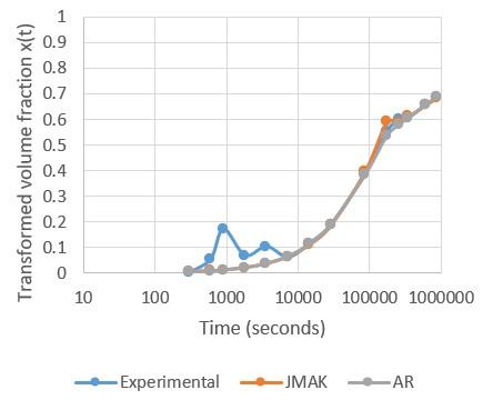
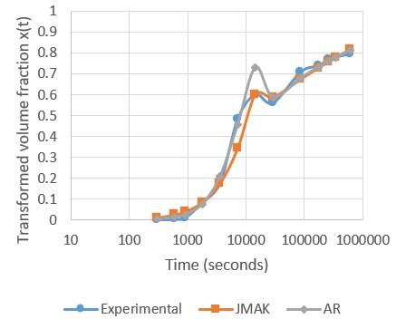
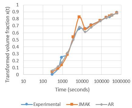
The two JMAK and AR models have now been identified. Therefore, the modellings obtained can be compared with the experimental values. Figure 6 shows the results on the 6082 alloy.
At 165℃, the two models rather faithfully convey the experimental data. There is a zone that is a little more complex to represent at the transition between the first and second transformation.
At 190℃, it can be seen that the zone of transition between the first transformation and the second transformation is still complicated to model. Secondly, it is the AR model that is the closest to the experimentally measured values given that the zone of transition is greatly overestimated. The JMAK model is firstly below the real value however it better reflects the zone of transition. For the two models, the second transformation is appropriately represented.
(a) 165℃
(b) 190℃
(c) 210℃
Figure 6. Comparisons of the JMAK and AR models with the experiment for the transformed volume fraction
At 210℃, it is yet again the zone of transition which is problematic, however it is the AR model which best conveys this. For the rest, the two models are fairly similar and close to the experimental values.
Thus, excluding the zone of transition, the two models offer good adjustments of the transformed volume fraction x(t).
3.3 Avrami exponent as a function of the temperature
As it can be seen (paragraphs 3.2.1 and 3.2.2) n is not a constant that is independent of the temperature. The equation connecting it to the temperature can be determined from n.
3.3.1 6082 alloy
- JMAK model:
1st transformation: $n=\frac{-1780.9}{T}+4.91$ (with a good determination coefficient R2>0.9)
2nd transformation: $n=\frac{154.1}{T}-0.13$ (with a poor determination coefficient R2≈0.75).
- AR model:
1st transformation: $n=\frac{-1079.4}{T}+3.3546$ (with a good determination coefficient R2>0.9)
2nd transformation: $n=\frac{-125.6}{T}+0.6591$ (with a poor determination coefficient R2≈0.27).
3.3.2 6061 alloy
- JMAK model:
1st transformation: $n=\frac{1194.8}{T}-1.484$ (with a good determination coefficient R2>0.9)
2nd transformation: $n=\frac{-489.8}{T}+1.187$ (with a poor determination coefficient R2≈0.82).
- AR model:
1st transformation: $n=\frac{-209.1}{T}+1.632$ (with a good determination coefficient R2>0.9)
2nd transformation: $n=\frac{-808.9}{T}+1.944$ (with a poor determination coefficient R2≈0.85).
Even if the correlation between n and T is not always perfect as shown by the previous equation, nevertheless it appears that n tends to evolve on a straight line basis as a function of 1/T.
3.4 Activation energy
By applying the Eq. (8), it is now possible to calculate the activation energy $E_{a}$ by plotting $\ln (k(T))$ as a function of $\frac{1}{R T}$. The slope of the line is therefore $E_{a}$. Table 4 shows the values obtained as well as the associated determination coefficient.
As stated in paragraphs 3.2.1 and 3.2.2., the first transformation kinetics conveys the precipitation of phase β’’ and phase β’. As such, the activation energies calculated correspond to the higher of the phase β’’ or phase β’ precipitation values (in general, this is the phase β’ precipitation value). The literature [17, 18], provides a few examples of values corresponding to the activation energy for the formation of phase β’: these values range between 105 kJ/mol and 145 kJ/mol. The values obtained with the two models are similar and are consistent with the data provided in literature, even if it can be noted that they are higher in our study. We also note that they are close to the Mg and Si diffusion values in aluminium, i.e. 131 kJ/mol and 124 kJ/mol respectively [19]. The second transformation kinetics is associated with the precipitation of phase β. We obtain rather heterogeneous activation energy values especially for the 6061 alloy where the value obtained with the JMAK model is more than twice that obtained with the AR model. If we refer to literature [20], the activation energy for the precipitation of phase β is approximately 225 kJ/mol, which is not consistent with our results.
Table 4. Activation energy of the 1st (1) and 2nd (2) transformation kinetics based on the JMAK and AR models
|
6082 |
JMAK |
AR |
||
|
(1) |
(2) |
(1) |
(2) |
|
|
$E_{a}$ (kJ/mol) |
149.9 |
149.7 |
146.2 |
125.7 |
|
R² |
0.99 |
0.99 |
0.99 |
0.97 |
|
6061 |
JMAK |
AR |
||
|
(1) |
(2) |
(1) |
(2) |
|
|
$E_{a}$ (kJ/mol) |
131.3 |
304.6 |
148.4 |
138.2 |
|
R² |
0.99 |
0.92 |
0.99 |
0.99 |
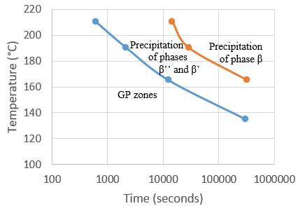
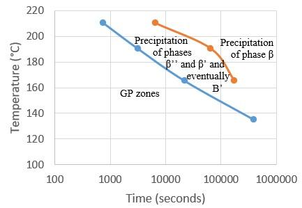
With the data obtained in this study concerning the two aluminium alloys, we can plot time – temperature – transformation (TTT) diagrams or more precisely time – temperature – precipitation (TTP) diagrams for each alloy. An example of the TTP diagram is presented in Figure 7 for alloy 6082 and in Figure 8 for alloy 6061. It should be highlighted that these are partial diagrams (zones of temperature studied). Moreover, note that the blue lines on Figures 7 and 8 show the start of precipitation for phases β’’ and β’ and the red lines the start of precipitation of phase β. These are not precipitate stability zones. With regard to the Guinier Preston zones (GP zones), we do not show the start of precipitation as the two diagrams are constructed based on isotherms carried out after 48 hours of natural ageing (Table 1): the GP zones have already begun to precipitate.
Figure 7. Alloy 6082 – partial TTP diagram
Figure 8. 6061 alloy – partial TTP diagram
According to Fang et al. [21], who investigated an alloy similar to the 6082: an Al-0.89Mg-0.75Si alloy with trace Fe and Zn elements, by transmission electron microscopy (TEM), the following results were noted:
If the TTP diagram for the 6082 is used, it can be noted that it predicts:
This is consistent with the TEM observations of Fang et al. [21] especially seeing that as previously stated, the studied alloy is not a 6082 alloy but a similar alloy.
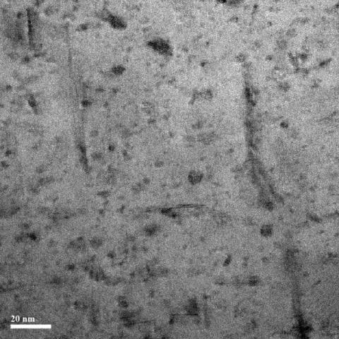
In Figure 9 which shows our TEM observation for 4 hours at 190℃ on 6061 alloys, numerous and very fine needle-shaped precipitates about 30 to 50 nm in length and 2 to 5 nm in diameter are observed. These precipitates are typically the phase β’’ [21]. This indicates that the diagram in Figure 8 is consistent with the experiment (at least for this temperature).
Figure 9. 6061 alloy – only phase β’’ (all shapes)
The electrical conductivity measurement method is easy to implement and sensitive to the changes in the precipitation state. We investigated the precipitation kinematics of two aluminium alloys, 6082 and 6061, during an isothermal transformation. The electrical conductivity is due to the contribution of the precipitates, the solid solution and defects. It is noted for the two alloys that the electrical conductivity increases during an isothermal treatment towards an asymptotic value which is probably the value of the annealing. On the other hand, it can be noted that the hardness is very easy to achieve and can be quickly analysed. However, it only provides an overall view of the precipitation. It is useful for supplementing the results of another investigation technique such as electrical conductivity. It will be recalled that the hardness reaches its maximum all the faster the higher the heat treatment temperature and the maximum hardness is all the higher the lower the heat treatment temperature.
It was seen that the JMAK and AR models can be applied and that this application serves to identify the parameters for each alloy. The two models provide a good representation of the precipitation kinematics of the 6082 and 6061 alloys. The advantage of the JMAK model is the possibility of using the Avrami exponent to understand the precipitation mechanics (information in Table 3). The precipitation mechanisms cannot be fully identified using only the electrical conductivity. Therefore, it was not possible to differentiate the precipitation of phase β’’ from phase β’ which has the same Avrami exponent. Note that the Avrami exponent is a function of the temperature and seems to change linearly with 1/T. We were able to determine the activation energies of the various transformation kinematics and to compare them with literature. It was observed that the results obtained are consistent with those for the first transformation kinematics (precipitations of phases β’’ and β’) and that they are fairly close to the diffusion values of Mg and Si in aluminum. Finally, the data from this study was used to construct two partial time – temperature – precipitation (TTP) diagrams which seem to be consistent with the observations reported in literature. These diagrams provide the community with a “correct” but incomplete prediction of the precipitation of phases β’’, β’ and β (main phases of the two aluminium alloys) in a temperature range that is widely used by industrial sectors.
The authors wish to thank CETIM (Centre Technique des Industries de la Mécanique – Technical Centre for the mechanical industries) for the funding and support provided for this study.
[1] Dubost, B., Sainfort, P. (1991). Durcissement par précipitation des alliages d’aluminium. Techniques de l’ingénieur, M240 v1.
[2] Johnson, W.A., Mehl, R.F. (1939). Reaction Kinetics in processes of nucleation and growth. Transactions of the American Institute of Mining and Metallurgical Engineers, 135: 416-441.
[3] Avrami, M. (1939). Kinetics of phase change. I general theory. The Journal of Chemical Physics, 7(12): 1103–1112. https://doi.org/10.1063/1.1750380
[4] Avrami, M. (1940). Kinetics of phase change. II transformation‐time relations for random distribution of Nuclei. The Journal of Chemical Physics, 8(2): 212–224. https://doi.org/10.1063/1.1750631
[5] Avrami, M. (1941). Granulation, phase change, and microstructure kinetics of phase change. III. The Journal of Chemical Physics, 9(2): 177–184. https://doi.org/10.1063/1.1750872
[6] Austin, J.B., Ricckett, R.L. (1939). Trans. Am. Inst. Min. Eng. https://classiccarcatalogue.com/AUSTIN%201939.html, accessed on March 12, 2020.
[7] Totten, G., Mac Kenzie, S. (2003). Handbook of Aluminum. New York: Marcel DEKKER, volume 2, 1310 pages. https://doi.org/10.1201/9780203912591
[8] Miao, W.F., Laughlin, D.E. (2000). Effects of Cu content and preageing on precipitation characteristics in aluminum alloy 6022. Metallurgical and Materials Transactions A, 31(2): 361–371. https://doi.org/10.1007/s11661-000-0272-2
[9] Guidelines for Measurement the Electrical Conductivity with the Fischerscope MMS PC, 2004.
[10] ASTM E 1004-99. Standard Practice for Determining Electrical Conductivity Using the Electromagnetic (Eddy – Current) Method. ASTM International, West Conshohocken, PA, 1999, https://doi.org/10.1520/E1004-99
[11] Yan, J. (2006). Strength modelling of Al-Cu-Mg type alloys. Th. Doct. Philosophy, Southampton. Faculty of Engineering, Science & Mathematics, 215 p.
[12] Christian, J.W. (1965). The Theory of Transformations in Metals and Alloys. Pergamon Press, Oxford.
[13] Malek, J. (1995). The application of Johnson – Mehl – Avrami model in the thermal analysis of crystallization, kinetics of glasses. Thermochimica Acta, 267: 61-73. https://doi.org/10.1016/0040-6031(95)02466-2
[14] Appolaire, B. Croissance/dissolution. Cours théorique de l’INPL. http://mms2.ensmp.fr/mat_nancy/croissance/transparents/6_croissance_r.pdf, accessed on Mar. 20, 2020.
[15] Røyset, J., Ryum, N. (2005). Kinetics and mechanisms of precipitation in an Al–0.2wt.% Sc alloy. Materials Science and Engineering: A, 396(1-2): 409–422. https://doi.org/10.1016/j.msea.2005.02.015
[16] Mulazimoglu, M.H. (1988). Electrical conductivity studies of cast Al-Si and Al-Si-Mg alloys. Th. Doct. Philosophy. Montréal. Departement of Mining and Metallurgical Engineering Mc Gill University, 249 p.
[17] Gaber, A., Gaffar, M.A., Mostafa, M.S., Zeid, E.F.A. (2007). Precipitation kinetics of Al–1.12 Mg2Si–0.35 Si and Al–1.07 Mg2Si–0.33 Cu alloys. Journal of Alloys and Compounds, 429(1-2): 167-175. https://doi.org/10.1016/j.jallcom.2006.04.021
[18] Hamdi, I., Boumerzoug, Z., Chabane, F. (2017). Study of precipitation kinetics of an Al-Mg-Si alloy using differential scanning calorimetry. Acta Metallurgica Slovaca, 23(2): 155. https://doi.org/10.12776/ams.v23i2.908
[19] Kinzoku data book Japan Institute of Metals, (1994). Sendai, Japan.
[20] Vedani, M., Angella, G., Bassani, P., Ripamonti, D., Tuissi, A. (2007). DSC analysis of strengthening precipitates in ultrafine Al–Mg–Si alloys. Journal of Thermal Analysis and Calorimetry, 87(1): 277–284. https://doi.org/10.1007/s10973-006-7837-2
[21] Fang, X., Song, M., Li, K., Du, Y. (2010). Precipitation sequence of an aged Al-Mg-Si alloy. Journal of Mining and Metallurgy, Section B: Metallurgy, 46(2): 171–180. https://doi.org/10.2298/jmmb1002171f